
GNSS Anti-Jamming PCB: CRPA Arrays, Multi-RF Isolation and Precision Timing
GNSS anti-jamming PCB design: CRPA array geometry at L1, the phase budget that sets null depth, multi-RF isolation, front-end loss and the 1 ns timing rules.
Home » Anti-Jam Antenna » GNSS Anti-Jamming PCB: CRPA Arrays, Multi-RF Isolation and Precision Timing
Table of Contents
A GNSS anti-jamming PCB is a board that has to do two jobs that pull in opposite directions: receive a signal about 30 dB below the thermal noise of its own band, and stay functional when something in the same band is 20 to 30 dB above it. Neither job is solved by the receiver chip alone. The antenna has to be an array so that it can place a null on the jammer, and the board underneath that array has to hold every channel to within a few degrees of phase, or the null never forms.
That is the whole engineering problem in one sentence, and it is a board problem before it is a signal-processing problem. At L1, one millimetre of trace is 3.11 degrees of phase. Three millimetres of length difference between two channels caps the achievable null at about 16 dB, no matter what the adaptive algorithm does afterwards. The numbers in this guide are all derived from that relationship: array geometry from the wavelength, phase budget from the length, null depth from the phase error, and the front-end loss budget from the noise figure it destroys.
The same board usually carries precision timing, and the second half of that requirement is harder than it looks: one nanosecond is 30 cm of range, and on a laminate with an effective permittivity of 2.7 a single millimetre of trace is 5.48 ps. Timing boards fail on connectors and filter group delay, not on the routing.
Array-level design theory sits in our phased array PCB review, the combining network in the corporate feed network guide, and the laminate landscape — parameter by parameter — in the high frequency PCB materials section. This page is the part that connects them: what the numbers have to be, and where they are decided.
1. The Threat Model: What Jamming and Spoofing Do to a Receiver Front End
Start with the signal budget, because every later number depends on it. A GPS L1 C/A signal at the antenna is about −130 dBm spread over 2.046 MHz. A receiver with a 2 dB noise figure has a noise density of −172 dBm/Hz. The correlator recovers about 43 dB of processing gain, which turns that into a usable carrier-to-noise density of 42 dB-Hz. Forty-two decibels is the entire margin between a working fix and no fix, and a jammer only has to close it.
Broadband noise jamming does that by lifting the noise floor. A 20 MHz noise source at −87 dBm puts a power density of −160 dBm/Hz at the receiver, 12 dB above thermal noise, and C/N0 falls from 42 to 30 dB-Hz. At −77 dBm the density is 22 dB above thermal and C/N0 is 20 dB-Hz, which is where most receivers stop tracking.
Narrowband jamming is more efficient per watt. The same receiver hit by a −110 dBm tone inside a 1 kHz bandwidth sees −140 dBm/Hz: 32 dB above thermal noise, from a source 20 dB weaker than the broadband jammer above. Power density is the currency, not total power, and it is why a cheap single-tone source can be more damaging than an expensive wideband one.
| Jammer | Total power / bandwidth | J0 at the receiver (dBm/Hz) | N0 + J0 (dBm/Hz) | C/N0 afterwards (dB-Hz) | Suppression needed for 40 dB-Hz |
|---|---|---|---|---|---|
| Broadband noise | −87 dBm in 20 MHz | −160.0 | −159.7 | 29.7 | 10.3 dB |
| Broadband noise | −77 dBm in 20 MHz | −150.0 | −150.0 | 20.0 | 20.0 dB |
| Narrowband noise | −100 dBm in 1 MHz | −160.0 | −159.7 | 29.7 | 10.3 dB |
| CW tone | −120 dBm in 1 kHz | −150.0 | −150.0 | 20.0 | 20.0 dB |
| CW tone | −110 dBm in 1 kHz | −140.0 | −140.0 | 10.0 | 30.0 dB |
Computed for a signal at −130 dBm, a receiver noise figure of 2 dB and N0 = −174 dBm/Hz + NF, i.e. −172 dBm/Hz. Unjammed C/N0 is 42 dB-Hz. Note that the −110 dBm CW tone is 20 dB weaker than the −87 dBm broadband source yet needs three times the suppression: what a receiver sees is power density, not total jammer power.
Spoofing is a different failure and cannot be nulled away. The false signal arrives from the satellite direction, exactly where the array is trying to listen, so an antenna pattern is no defence. What an array can do is compare the phase across elements and check whether the apparent direction of arrival is consistent with the ephemeris; a single-element receiver has nothing to compare. That is a second, independent reason to put more than one element on the board, and it is worth designing the channel matching for it even when jamming is not the primary requirement.
The last column of the table is the specification the antenna has to meet, and it is a phase-error specification in disguise. An array with M elements has M−1 degrees of freedom and can place that many independent nulls; a four-element array has three, a seven-element array has six. What it cannot do is place a null deeper than the channel matching allows, which brings the whole problem down to millimetres of trace.
2. CRPA Array Geometry and the Phase Budget Behind Null Depth
Geometry starts from the free-space wavelength: 190.29 mm at L1, 244.21 mm at L2 and 254.83 mm at L5. On a 0.508 mm laminate with a dielectric constant of 3.4, a 50 Ω microstrip line is 1.18 mm wide and presents an effective permittivity of about 2.7, so the guided wavelength at L1 is 115.8 mm and a resonant patch length falls near 57.9 mm. The patch figure is an estimate until the stackup is fixed; the wavelength and the line width are not.
Element spacing is bounded from above by grating lobes and from below by mutual coupling. For a scan to ±60° the limit is d ≤ λ0/(1 + sin 60°) = 102 mm, which at L1 is 0.536 λ0. Half a wavelength, 95.1 mm, sits just inside that, and this is why CRPA layouts look crowded: there is no room to space the elements for isolation without giving up scan range. At ±45° the limit relaxes to 111.5 mm, which buys 16 mm per element pair and a noticeably easier feed.
| Array | Elements | Spacing | Nulls (M−1) | Aperture | Board footprint |
|---|---|---|---|---|---|
| 2 × 2 square | 4 | 95.1 mm (0.50 λ0) | 3 | 153 mm | ≈ 184 × 184 mm |
| 7-element hexagonal | 7 | 95.1 mm (0.50 λ0) | 6 | 248 mm | ≈ 298 × 298 mm |
| 7-element hexagonal | 7 | 104.7 mm (0.55 λ0) | 6 | 267 mm | ≈ 321 × 321 mm |
L1 at 1575.42 MHz: λ0 = 190.29 mm. Aperture is measured across the array including the element itself (λg/2 = 57.9 mm at εeff 2.7). The footprint allows 20 % for the fence, connectors and mounting keep-out. Spacing beyond about 0.54 λ0 starts to cost scan range at L1.
Then comes the part that decides whether the array works. The phase of a 100 mm line at L1 is 310.9°, so one millimetre is 3.11°. Null depth is limited by the phase error between channels according to 20·log10(Δφ in radians): 1 mm of mismatch, 3.1°, supports about 25 dB; 3 mm, 9.3°, supports 16 dB; 5 mm, 15.5°, supports 11 dB. Amplitude errors do the same thing from the other side — a 0.5 dB imbalance limits the null to about 25 dB, 0.2 dB to about 33 dB — which is why the feed is built from Wilkinson dividers rather than from a tapered tree that happened to fit.
| Contributor | On the drawing | Phase at L1 (100 mm line) | How it is held |
|---|---|---|---|
| Layout length difference | per millimetre | 3.11° | Equal-length routing with a defined reference plane |
| Laminate Dk tolerance | ± 0.05 on 3.4 (± 1.5 %) | ± 1.60° | Lot certificate plus one panel per build measured on a coupon |
| Dielectric thickness | ± 0.05 mm on 0.508 mm | ± 1.10° | Thickness tolerance in the purchase spec, not the default |
| Etch tolerance | ± 25 µm | ± 0.08° | Standard imaging |
| Thermal gradient | 10 °C across the panel | ± 0.12° | Thermal isolation from the power amplifier |
| Connector launch | per port, measured | ± 2° (allocation) | Same connector family, same launch geometry on all channels |
| Cable / assembly match | per channel, measured | ± 3° (allocation) | Phase-matched harness, measured before installation |
The line is 310.9° long per 100 mm at L1, so everything that changes its length or its effective permittivity lands directly on the null. Root-sum-square of the three material terms is about 2°, which means the layout term decides the result: 3 mm of extra trace is 9.3° and caps null depth at 16 dB before any material effect is counted.
There is a trap in multi-band arrays that single-band design rules do not catch. The phase per millimetre is not the same at the three frequencies: 3.11° at L1, 2.42° at L2, 2.32° at L5. A physical offset introduced to correct an L1 phase error therefore leaves L2 wrong by 0.7° per millimetre of offset. Over a 20 mm routing difference, that is 14° of L2 phase error — a 17 dB null at L1 and a 12 dB null at L2 from the same board. The only geometry that holds all three bands at once is equal physical length in the same medium; where that is impossible, the correction has to be per band, not per millimetre.
Two practical consequences follow. First, the reference plane for "equal length" has to be defined before routing starts, usually at the centre of the array or at the common port of the combiner, because length measured from a different point produces a different answer on every channel. Second, length matching is the cheap part: ± 0.1 mm of routed length is 0.3°, well inside any reasonable budget. The expensive part is the launch, where a connector transition contributes a couple of degrees on a good day and considerably more on a bad one.
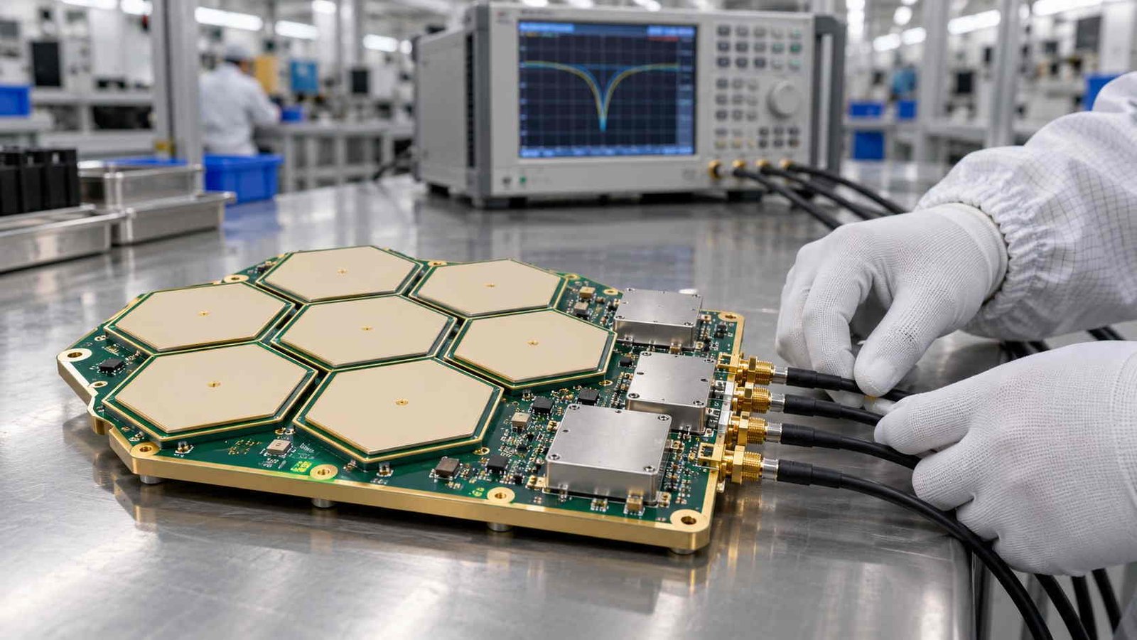
3. Multi-RF Coexistence: Isolation, Filtering and Ground Partitioning
Almost no GNSS board is alone. The same product usually carries an LTE or 5G modem, a Wi-Fi radio and a switching supply, and the GNSS front end is the most sensitive circuit on the assembly by two orders of magnitude. What saves it is not layout care in general but a specific isolation number per aggressor, computed from the transmitter power, the antenna separation and the linearity of the first amplifier.
The arithmetic is short. A 33 dBm transmitter one metre away produces −4.8 dBm at the GNSS antenna at 1.84 GHz after 37.8 dB of free-space loss. With 20 dB of antenna-to-antenna coupling — the figure to assume until it is measured, and optimistic at half-wavelength separation — the LNA sees −24.8 dBm. To keep the front end out of compression and out of third-order mixing, that has to come down to about −50 dBm, so 25 dB of rejection is needed at that offset.
| Co-located source | Frequency | Offset from L1 | Level at the GNSS antenna | Level at the LNA input | Rejection needed |
|---|---|---|---|---|---|
| LTE 1800 downlink | 1842.5 MHz | + 267 MHz | −4.8 dBm | −24.8 dBm | 25 dB |
| Wi-Fi 2.4 GHz | 2442 MHz | + 867 MHz | −7.2 dBm | −27.2 dBm | 23 dB |
| LTE 2600 downlink | 2655 MHz | + 1080 MHz | −7.9 dBm | −27.9 dBm | 22 dB |
| 5G n78 | 3500 MHz | + 1925 MHz | −10.3 dBm | −30.3 dBm | 20 dB |
| LTE 700, 2nd harmonic (30 dBc) | 1575.4 MHz | in band | −27.4 dBm | −47.4 dBm | not filterable |
Computed for a 33 dBm EIRP transmitter at 1 m, free-space loss of 37.8 dB at 1.84 GHz, and −20 dB antenna-to-antenna coupling. Rejection is what it takes to bring the LNA input down to −50 dBm. Replace the coupling figure with the measured value before the numbers are used in a link budget: at half a wavelength separation, two resonant elements couple far worse than −20 dB.
Why −50 dBm and not −30? Because of third-order intermodulation. With an input intercept point of −10 dBm, two tones at −50 dBm generate a product at 3(−50) − 2(−10) = −130 dBm, which is at the noise floor and harmless. Two tones at −30 dBm generate −70 dBm, forty decibels above the noise floor, and that lands in band where no filter can remove it. The pre-filter is not there to protect the antenna; it is there to keep the amplifier linear.
One case has no filter solution at all. The second harmonic of 787.71 MHz is 1575.42 MHz — exactly L1. If a 700 MHz transmitter on the same platform has insufficient harmonic suppression, the product is in band and indistinguishable from signal as far as the GNSS chain is concerned. It has to be suppressed at the transmitter output, and the board-level defence is only to keep the two antennas apart and the transmitter's output filter specified. This is the coexistence item most often missed in a design review, because the two radios are in different subsystems and nobody owns the interface.
Ground partitioning completes the isolation budget. The array needs one continuous ground plane under all elements, not a split plane with a single tie: a split under a radiator turns the gap into a slot radiator and shifts the resonance. Digital and switching returns belong on their own layer and must not cross under the array; the shield can goes down with a via fence at λ/20 spacing, 9.5 mm at L1, and the fence has to be continuous at the can gasket, not only at the corners. The GNSS supply comes from a linear regulator, not from the switching rail that feeds the modem. Details of what a via fence does to a radiating edge are in our phased array PCB article; the drill-side limits of a 0.2 mm fence pitch are on the high frequency PCB drilling capabilities page.
4. Feed Loss: Why 0.3 dB Is Not a Rounding Error
Everything between the radiating element and the first transistor is subtracted from the noise budget and nothing downstream can put it back. The Friis cascade says it plainly: a passive loss of L dB ahead of an amplifier with a 1.0 dB noise figure produces a system noise figure of L + 1.0 dB. The penalty is exactly one for one, in decibels, with no gain to dilute it.
| Loss ahead of the LNA | NF added | Noise temperature added | Jammer margin lost |
|---|---|---|---|
| 0.1 dB | + 0.10 dB | + 9.5 K | 0.1 dB |
| 0.3 dB | + 0.30 dB | + 29.2 K | 0.3 dB |
| 0.5 dB | + 0.50 dB | + 49.8 K | 0.5 dB |
| 1.0 dB | + 1.00 dB | + 105.7 K | 1.0 dB |
| 2.0 dB | + 2.00 dB | + 238.7 K | 2.0 dB |
Friis cascade with a 1.0 dB LNA and 20 dB gain. Every tenth of a decibel in front of the LNA arrives in the system noise figure unchanged — there is no downstream gain that recovers it. For scale, the sky noise at L1 is already around 100 K, so 0.5 dB of board loss adds half as much noise again as the whole sky.
The same number appears twice more. In noise temperature, 0.3 dB of loss is 29 K, and at L1 the sky already contributes around 100 K, so a half decibel of board loss adds half as much noise again as the entire sky. In jammer margin, 0.3 dB of loss is 0.3 dB off the J/S threshold — which is the same 0.3 dB that the array spent three millimetres of length matching to recover. Loss and phase are not separate budgets on this board; they are the same budget.
A realistic front-end allocation that holds the total near 0.55 dB looks like this: element and matching 0.05 dB, feed and combiner 0.25 dB, connector 0.10 dB, pre-filter 0.15 dB. Every line in that list is a fabrication and component decision, which is why the loss figure belongs in the RFQ and not in a note attached to the Gerbers. The same discipline is covered from the trace side in our 50 ohm RF trace guide and from the impedance side in controlled impedance RF PCB.
One architectural decision dominates the allocation: whether the LNA sits at the element or after the combiner. A four-way corporate feed has 6 dB of splitting loss. If the amplifier is after the combiner, those 6 dB land in the noise figure and the array is 6 dB deafer than it needed to be. Put the amplifier at the element and only its own 0.05 dB of matching loss counts; the combining network then runs at a comfortable power level where its loss affects dynamic range, not sensitivity. This is also why the feed on a receive array is usually stripline rather than microstrip — the shielded line matters more than the fraction of a decibel it costs, and the comparison is set out in microstrip vs stripline.

5. Precision Timing: 1 ns, 30 cm and What It Does to the Layout
A timing receiver is judged on a different axis from a navigation receiver. Navigation needs a few nanoseconds; time transfer needs about one, and PTP-class distribution on the board needs a hundred picoseconds. One nanosecond of error is 30 cm of apparent range, and the conversion is worth keeping in view because it never gets better: no amount of averaging removes a length error that is stable.
On the board the scale is tighter than intuition suggests. At an effective permittivity of 2.7 the propagation velocity is 1.825 × 10⁸ m/s, so one millimetre of trace is 5.48 ps and one picosecond is 0.18 mm. A clock tree matched to 10 ps is matched to 1.8 mm, which is easy. The difficulty is not the routing tolerance; it is everything the routing cannot see.
| Quantity | In air | On the board (εeff 2.7) | What it buys |
|---|---|---|---|
| 1 ns | 30.0 cm | 18.2 cm | Pseudorange; navigation-grade agreement |
| 100 ps | 3.0 cm | 1.8 cm | PTP-class time distribution |
| 10 ps | 3.0 mm | 1.8 mm | A matched clock tree |
| 1 ps | 0.30 mm | 0.18 mm | The resolution of a good VNA |
| 1 mm of trace | 3.34 ps | 5.48 ps | One millimetre is not free |
Propagation in the laminate runs at c/√εeff = 1.825 × 10⁸ m/s, so the board is electrically longer than the same length in air by a factor of 1.64. Every timing number below is quoted in board length on purpose: that is the unit a layout is checked in.
The reference plane is the first hidden term. A clock trace that crosses a plane split does not stop at the split — its return current detours around it, and the detour adds several millimetres of effective path plus a lumped discontinuity, which shows up as tens of picoseconds and as jitter. The rule on a timing board is stricter than on a data board: no signal crosses a split, and the reference plane for the timing domain is continuous from the oscillator to the last destination, even if that means giving the plane its own layer.
The second hidden term is the front-end filter. A SAW filter's group delay varies with temperature, typically by more than a nanosecond over the industrial range, and one nanosecond of group delay drift is 30 cm of apparent range that no calibration can remove unless the temperature is measured at the filter. For a timing receiver, ask for the group delay versus temperature curve before asking for insertion loss: the loss costs a fraction of a decibel, the drift costs the specification. Connector phase stability is the third term and is usually larger than the PCB contribution by an order of magnitude.
Thermal design closes the loop. On the PCB the effect is small — a 10 °C gradient across the panel moves the phase of a 100 mm line by 0.12°, about 0.2 ps — but the same gradient across a filter or a cable assembly is a different order of magnitude. Thermal isolation of the GNSS section from the power amplifier is therefore a timing measure as much as a noise measure, and it is the reason the oscillator sits away from the transmit chain even when the layout would prefer otherwise.
6. Laminate and Stackup: The Parameters That Move the Null
A CRPA board does not need an exotic laminate; it needs a specified one. The distinction matters, because the failure mode on this board is not "too much loss" but "two channels that disagree". That makes Dk tolerance and Dk uniformity across the panel the first two rows of the requirement list, ahead of loss tangent, which is the parameter most often discussed.
| Parameter | What it moves on a CRPA board | Number at L1 | Requirement |
|---|---|---|---|
| Dk tolerance | Channel-to-channel phase | ± 1.60° per 100 mm for ± 0.05 on 3.4 | Tight, and uniform across the panel |
| Dk uniformity within a panel | Null depth between neighbouring elements | Same term as above | Panel-level spread, not just lot tolerance |
| TCDk | Element resonance | 3.59 MHz over 60 °C at −110 ppm/°C | Flat over the operating range |
| Df | Feed and element loss | Counts 1:1 against NF | As low as the loss budget requires |
| CTE, z axis | Plated barrel strain through assembly | Multiplied by the stackup height | Compatible with the rest of the stack |
| Moisture absorption | Resonance drift outdoors | Scales with absorbed water | Low, for any outdoor unit |
| Thickness tolerance | Z0 and εeff | ± 0.05 mm on 0.508 mm → ± 1.10° per 100 mm | Tight and uniform |
Read this table as a requirement list, not as a material ranking. A grade satisfies the requirement or it does not; which grade that is depends on the band, the stackup and the thermal budget of the specific board, and it is a decision made with the numbers, not against a brand.
Put numbers on the first three rows. A Dk tolerance of ± 0.05 on 3.4 is ± 1.5 %, which moves the phase of a 100 mm line by 1.6° — inside a 3° channel budget, but only just, and only if every channel comes from the same panel. The temperature coefficient is a different kind of term: at −110 ppm/°C, a 60 °C excursion changes Dk by 0.66 %, which pushes a patch resonance up by 5.2 MHz while thermal expansion of the element pulls it back down by 1.6 MHz, for a net 3.6 MHz. Against the 2.046 MHz C/A bandwidth, that is the difference between a tuned element and a detuned one, and it is why element dimensions are confirmed at temperature rather than at 25 °C.
Stackup comes next. A GNSS board is usually a hybrid: microwave laminates for the array and the feed, FR-4 for the digital, power and connector layers. That combination is normal and it works, but the interface is where builds fail — registration between the two materials, z-axis CTE difference through the plated barrels, and warp on a 300 mm panel. The parameter comparison behind that decision is in mixed laminate FR4 Rogers, the fabrication detail in FR4 Rogers hybrid PCB, and the material families — parameter by parameter — in the Rogers materials and PTFE materials sections.
Two specific grades come up often enough to name as reference points, not as recommendations: RO4003C for a glass-reinforced hydrocarbon stackup and RO3003 for a PTFE-based one. Both are specified by their published parameters, and which of them — or neither — satisfies a given requirement depends on the band set, the stackup height and the thermal budget of the specific board.
7. Fabrication and Acceptance: What to Measure, What to Reject
An RF fabrication quote normally states impedance to ± 5 % and stops there. On a CRPA that is half a specification: ± 5 % absolute is achievable, but four channels that each hit 50 Ω within 5 % can still disagree with each other by 3 Ω, and the array only cares about the disagreement. The requirement to write into the purchase order is a channel-to-channel spread, measured on the same coupon, in the same fixture, on the same day.
| Check | Method | Criterion |
|---|---|---|
| Absolute impedance | TDR coupon, one per channel | 50 Ω ± 5 % |
| Channel-to-channel impedance spread | The same coupon, all four or seven traces | ≤ 1 Ω between channels |
| Channel phase | 4-port VNA, common reference plane, 1.575 GHz | ≤ 3° spread → 26 dB null capability |
| Routed length against the drawing | Optical measurement on the etched coupon | ± 0.1 mm (≈ 0.3°) |
| Launch quality | TDR at the coaxial port | No discontinuity above 5 Ω |
| RF-to-FR4 registration | Cross-section, three points per panel | ± 75 µm |
| Solder mask over radiators | Drawing plus AOI | Mask-free radiating area, or the effect is in the model |
| Surface finish | XRF thickness | Specified on loss and PIM, not on price |
| Warp | Flat-plate measurement after reflow simulation | ≤ 0.5 % on a 300 mm panel |
The first two rows are the ones a generic RF fab quote will not mention. Absolute impedance to ± 5 % is normal; four channels that agree with each other to within 1 Ω is the requirement a CRPA actually has, and it is a different process control problem.
Phase is measured, not inferred. The method that works is a four-port VNA with a common reference plane, all channels measured in one connection sequence so that cable drift cancels, at the operating frequency rather than at 1 GHz. Put a four-channel phase coupon on the panel edge — the same length and the same launch as the real channels — and measure it on the first article and on one panel from each lot. A phase spread of 3° corresponds to a 26 dB null; a spread of 10° corresponds to 15 dB, and that is a reject, not a note.
Solder mask belongs in the drawing, not in the default process. Mask over a radiating element shifts its resonance measurably, and on a 58 mm patch the shift is larger than the Dk tolerance term. Either the radiating area is mask-free by drawing, or the mask is in the model — but it cannot be left to whichever panel the shop had in the etcher that day. The same logic applies to the surface finish: it is specified on loss and passive intermodulation, not on price, and the finish under a radiating element is part of the RF design.
Back drilling is a smaller term at L1 than at 3.5 GHz — a 0.5 mm stub is not the limiting discontinuity at 1.6 GHz — but the same via often carries the 5G radio on the same board, and then the stub matters at the higher frequency. It is cheaper to specify the drill schedule once, for the highest band on the assembly, than to add it after the first prototype. What the line can hold on stub length and drill pitch is described in high frequency PCB drilling capabilities, and the module-level assembly consequences are in antenna module PCB assembly.
8. Design Review Checklist and Common Failure Modes
New on this subject
- multi-band counter-UAS jammer PCB — band-dedicated chains, sealed-shell dissipation and co-site isolation
The failure modes on this kind of board are unusually predictable, which is good news: almost all of them are decided in the first week of layout and almost none of them are discovered until the array is measured. The table below is the list we work through with customers before a build, ordered by how often it is the actual cause.
| Symptom | Most likely cause | Where to fix it |
|---|---|---|
| Nulls form but never deeper than about 15 dB | Channel length mismatch above 3 mm, or unequal launches | Layout and launch geometry |
| Null depth varies between builds of the same design | Dk spread between panels, or mask left on some radiators | Material certificate and fabrication drawing |
| Null drifts when the transmitter keys up | Thermal gradient from the power amplifier | Thermal isolation, copper balancing |
| C/N0 collapses only when the LTE radio transmits | LNA saturation or an in-band harmonic | Pre-filter, transmitter harmonic suppression |
| Resonance sits 3–4 MHz high in the field | Dk temperature coefficient plus thermal expansion | Element tuning at temperature, not at 25 °C |
| Timing steps by about 1 ns between units | Connector or cable phase, filter group delay | Harness specification |
| Position solution jumps without a C/N0 drop | Spoofing | Not a board issue — cross-check angle of arrival |
Everything in the right-hand column is decided before fabrication except the last row, which is decided by whether the receiver is allowed to compare phase across elements at all.
Three questions are worth asking before the Gerbers are released. Is the length reference plane defined, and does every channel measure from it? Is the pre-filter ahead of the amplifier, and does its rejection hold at the specific offset rather than at the band edge? And is the array's ground continuous under every element, with no digital return crossing beneath it? A board that answers yes to those three has a chance of reaching its null depth; one that does not will be debugged in the chamber, at the end of the schedule.
If the design is still at the material-selection stage, the parameter comparisons are in our PCB material comparison chart and the definitions behind them in the high frequency PCB glossary. For UAV and other space-constrained platforms, where the array and the modem share the same enclosure, the mechanical and thermal constraints are covered in UAV unmanned systems PCB. Fabrication capability for the whole assembly is summarised on the RF PCB manufacturer page.
GNSS Anti-Jamming PCB — Frequently Asked Questions
Element count, laminate parameters, coexistence with a cellular radio, and the length tolerance that decides null depth.
What makes a GNSS board anti-jamming — isn't that the antenna's job?
The array is the antenna, but the null depth comes from the board. A controlled reception pattern antenna steers a null toward the jammer by weighting the phase and amplitude of each element, and the weights can only be as accurate as the channels are matched. At L1 one millimetre of trace is 3.1 degrees, so a three-millimetre length error caps the achievable null at about 16 dB, whatever the digital signal processing does afterwards. That is why a CRPA is a layout problem before it is an algorithm problem.
How many elements do I need for a CRPA?
One more than the number of independent directions you need to suppress. A four-element array has three degrees of freedom: enough for one jammer plus the two strongest multipath replicas of it. A seven-element hexagonal array has six, which is what most multi-constellation receivers use when they have to hold a fix while a directional jammer sweeps. The cost is size: 184 mm square for four elements, 298 mm square for seven at L1 with half-wavelength spacing.
Can a GNSS receiver share a board with an LTE or 5G radio?
Yes, with a quantified isolation budget rather than a hopeful layout. A 33 dBm transmitter one metre away puts about −5 dBm at the GNSS antenna at 1.8 GHz and about −25 dBm at the LNA input after 20 dB of antenna-to-antenna coupling. Bringing that to −50 dBm needs roughly 25 dB of rejection ahead of the LNA, which a filter can supply if it sits in front of the amplifier and not behind it. The one case no filter solves is the second harmonic of the 700 MHz band, which lands exactly on L1 at 1575.42 MHz and has to be suppressed in the transmitter.
Which laminate should a CRPA board use?
The one that meets the parameter list, which is a design decision rather than a default. What the board needs is a Dk tolerance tight enough to keep channel phase inside the null budget, a Dk that stays flat over temperature, a loss tangent low enough for the front-end allocation, and a thickness tolerance that holds 50 Ω across the panel. Those four numbers, plus the CTE of whatever else is in the stackup, decide the grade. Any laminate that meets them will build a working array; the parameter list is what to compare against.
What length tolerance should I specify on a CRPA feed?
Work backwards from the null depth. Thirty degrees of channel phase error buys about 6 dB of null, ten degrees buys 15 dB, three degrees buys 26 dB. At 3.11 degrees per millimetre at L1, that is a millimetre-scale requirement, not a mil-scale one — so specify ± 0.1 mm of routed length, and spend the effort on the launch and the connector instead, where the phase error is larger and much harder to control.
Building a CRPA or a timing board?
Send us the band set, the element count and the stackup you have in mind. We will confirm the achievable channel phase spread before the layout is frozen, agree which Dk figure goes into the impedance target, and quote fabrication with coupon TDR and four-port phase data on the lot we actually build from.
Contact Us → WhatsApp: +86 137 6047 3650Request a PCB Quote
Upload your Gerber ZIP file and project requirements. Our engineering team will review your PCB material, stackup, impedance needs, surface finish, and production quantity before quoting.
Please prepare:
- Gerber files in ZIP format
- PCB material or stackup requirements
- Controlled impedance notes if available
- Prototype or batch production quantity