
PTFE Backplane PCB: Manufacturing Limits for 1-Metre AI Data-Center Boards
PTFE backplane PCB manufacturing: 1-metre loss budgets at 28 and 56 GHz, lamination and drilling limits, stub resonance, thermal growth and the tolerance that owns the impedance window.
Home » AI Data Center PCB » PTFE Backplane PCB: Manufacturing Limits for 1-Metre AI Data-Center Boards
Table of Contents
AI data-center hardware has outgrown the cable. Analyst coverage of Rogers' September investor day describes midplane and backplane boards up to a metre long and 24 to 72 layers replacing copper interconnect between servers and accelerators, with each material generation buying 10–20 % less insertion loss — and a new PTFE-based CCL exceeding current M9-class performance now sampling to head customers and their PCB partners. Whatever the exact product timeline, the direction is unambiguous: the loss budget of a one-metre channel is the new specification, and it is pulling PTFE-class laminates out of their millimetre-wave niche into boards the size of a forearm.
That migration collides with everything PTFE is famous for being bad at: it is soft, it presses and drills differently from glass epoxy, and a 24–72 layer stack leaves no room for process habits inherited from FR-4. This page works the problem as numbers, from one stated model: what a metre of channel loses at the 112G and 224G Nyquist frequencies, what PTFE actually buys, what the press and the drill have to pay, and which tolerances own the impedance and the skew. Every figure is computed, and the model assumptions are stated where they are used.
Material parameters for the laminate families — Dk, dissipation factor, CTE — are compared in the high frequency PCB materials section, with the PTFE family in PTFE materials and the ceramic-filled and hydrocarbon families in Rogers materials. This page is about what a fabrication line does to those numbers when the board is a metre long.
1. What a 1-Metre, 24–72 Layer Board Actually Is
The reported class of board — up to a metre long, 24 to 72 layers, carrying 112G and 224G-PAM4 serdes traffic between the accelerators — changes the scale of every manufacturing term. The table below translates the layer counts into the geometry a fabricator actually sees.
| Layer count (reported class) | Board thickness at these averages | Average dielectric layer | What the thickness implies |
|---|---|---|---|
| 24 layers | 3.2 mm | 133 µm | 12.8:1 aspect at a 0.25 mm drill |
| 36 layers | 4.0 mm | 111 µm | 16:1 aspect at the same drill |
| 48 layers | 4.8 mm | 100 µm | 19.2:1 aspect — sequential or laser options enter |
| 72 layers | 6.4 mm | 89 µm | 25.6:1 aspect — plating, not drilling, becomes the limit |
Geometry implied by the reported 24–72 layer class and 1-metre length — the layer counts are reported, the thicknesses are what uniform averages produce, not a datasheet. The fourth column is the point: at these thicknesses a full-length through hole is a stub whose first resonance sits far below the 28 GHz Nyquist of a 112G-PAM4 channel (section 4), so backdrilling or blind/laser stacks are not options, they are the architecture. Press and registration at 89–133 µm per layer across a 1-metre panel is section 3.
Two consequences follow immediately. First, thickness: at 89–133 µm per dielectric layer, registration across hundreds of layers-worth of image-and-etch steps happens at tolerances the FR-4 world associates with flex circuits — on a panel the size of an oven door. Second, the via architecture is decided before routing starts: a full-length through hole on a 3.2 mm board is a resonant stub half a band below the Nyquist (section 4), so the RF-relevant layers live on backdrilled or blind paths from the first revision, not as a cost-out after the first article.
The third consequence is the one nobody quotes: at these lengths the board is a transmission system. Five point eight nanoseconds of delay per metre, 58 degrees of phase per millimetre at 28 GHz — sections 2, 4 and 5 put numbers on what that does to loss, stubs and skew.
2. The Loss Budget of a One-Metre Channel
Loss on a metre-scale channel is two mechanisms with different owners. Dielectric loss scales with frequency and loss tangent — it belongs to the laminate. Conductor loss scales with surface resistance and roughness — and on backplane geometries it belongs to the stackup: line width and plane spacing decide it long before the laminate grade does. The table splits them for a stated 50 Ω stripline model.
| 50 Ω stripline model (εr 3.00, b = 0.51 mm) | 28 GHz (112G Nyquist) | 56 GHz (224G Nyquist) | Per inch at 28 GHz |
|---|---|---|---|
| Dielectric only (Df 0.0013) | 5.7 dB/m | 11.5 dB/m | 0.15 dB |
| Conductor, w = 0.153 mm nominal | 88 dB/m | 125 dB/m | 2.2 dB |
| Total, nominal line | 94 dB/m | 137 dB/m | 2.4 dB |
| Total, wide line w = 0.300 mm | 51 dB/m | 76 dB/m | 1.3 dB |
Computed, not measured. Model: symmetric 50 Ω stripline, εeff = εr; dielectric loss from the standard αd = π·f·√εr·tanδ/c; conductor loss from the flat-plate surface resistance times a 1.8 geometry factor (two planes plus sidewalls) times a Groiss roughness factor of 2.0 for an Rz 2 µm HVLP foil. The story is the second row: on a 0.51 mm stripline geometry the 50 Ω line is 0.153 mm wide, and copper — not the laminate — owns roughly nine tenths of the budget. Doubling the line width removes about half the total. The laminate class shifts the dielectric row (table 3); the geometry row is a stackup decision.
| Laminate class (εr / Df) | Dielectric loss at 28 GHz | At 56 GHz | Share of the nominal-channel budget |
|---|---|---|---|
| PTFE-class (3.00 / 0.0013) | 5.7 dB/m | 11.5 dB/m | ≈ 6 % of 94 dB/m |
| Low-loss hydrocarbon (3.48 / 0.0037) | 17.6 dB/m | 35.2 dB/m | ≈ 19 % of its own total |
| FR-4 (4.30 / 0.0200) | 106 dB/m | 211 dB/m | Listed for scale only |
Dielectric term only, from the same closed-form αd — exact within the model, no roughness assumptions involved. Over one metre the PTFE-class row spends 5.7 dB at the 112G Nyquist and 11.5 dB at the 224G Nyquist; the hydrocarbon row spends three times that; FR-4 spends more than the entire channel budget three times over. This is the row material selection controls. What it does not control is the conductor row in table 2 — which is why a laminate change alone never halves a backplane loss budget.
Read the two tables together. The dielectric rows are material selection, and over a metre the spread between a PTFE-class laminate and a low-loss hydrocarbon is 12 dB at the 112G Nyquist — decisive, and the reason the midplane migration points at PTFE-class materials. But the conductor row on the nominal 0.153 mm line is 88 dB/m: fifteen times the PTFE dielectric term. Doubling the line width — a stackup decision — removes roughly half of the total channel budget, which no realistic laminate change can match. The practical sequence is therefore: fix the geometry first, then buy the dielectric class the remaining budget asks for.
How those material parameters translate into design values — and how to read a datasheet before committing them to a metre of copper — is set out in the simulation-ready material data guide, and the side-by-side parameter trade-offs in the PCB material comparison chart.
3. Lamination and Dimensional Stability on a Metre-Scale Panel
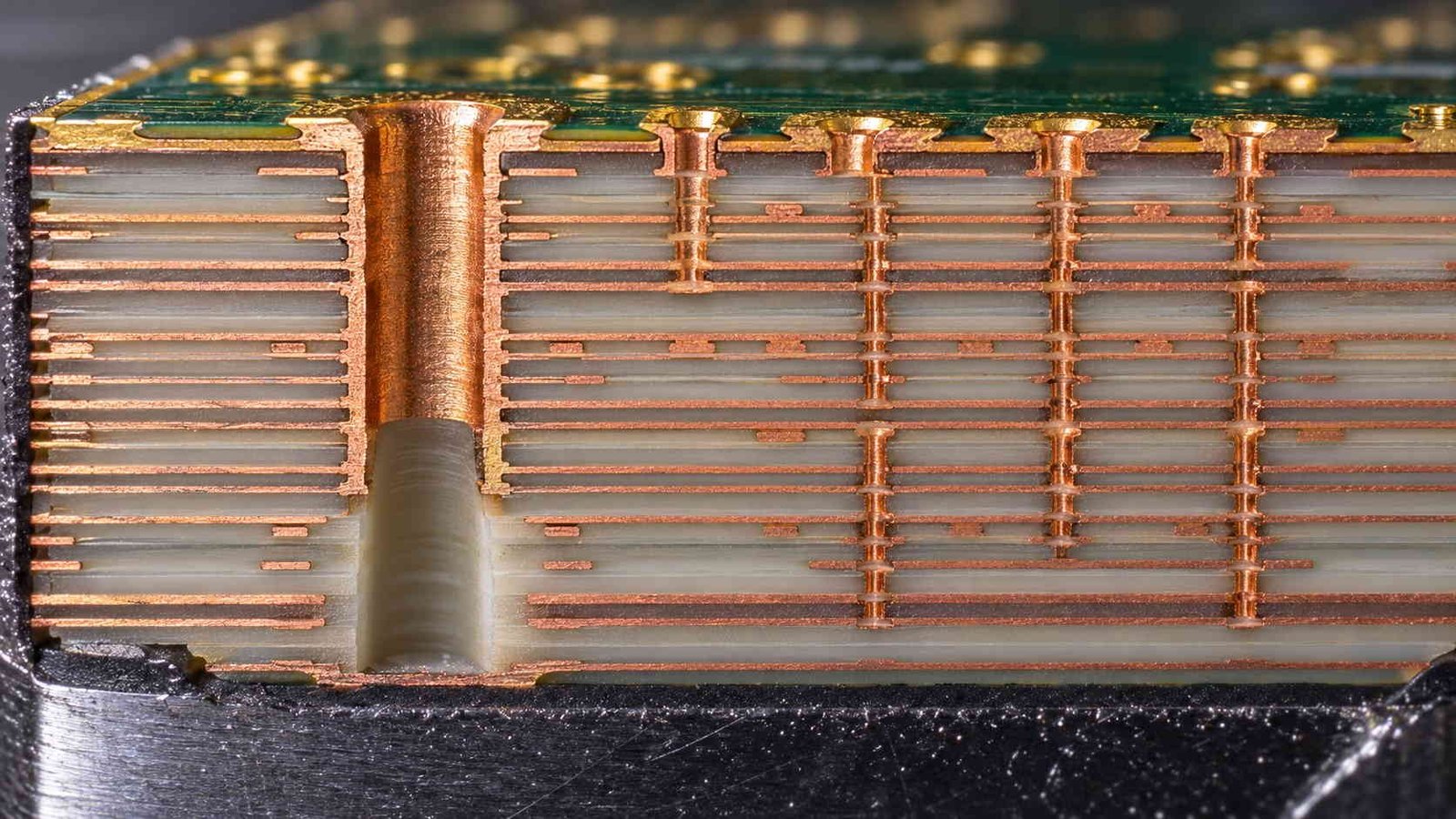
PTFE's electrical superiority comes with a mechanical personality the press has to manage: the base resin is soft, laminates flow and relax differently from glass-epoxy systems, and press cycles — pressure, ramp, cool-down — are qualified per material family, not shared. On a 24–72 layer stack, cool-down is also when the innerlayers register: the xy expansion of each layer during the thermal cycle becomes the permanent misalignment the drilling has to hit. That is why the expansion table below is a lamination parameter as much as a thermal one.
| ΔT (assembly to operation) | xy growth on a 1.0 m PTFE-class panel | z-axis growth on a 3.2 mm board | Context |
|---|---|---|---|
| 10 °C | 0.17 mm | 1.4 µm | Resoldering cycle window |
| 30 °C | 0.51 mm | 4.3 µm | Enclosure seasonal swing |
| 60 °C | 1.02 mm | 8.6 µm | A millimetre of length into the connector field |
xy CTE 17 ppm/°C and z CTE 45 ppm/°C (ceramic-filled PTFE-class datasheet values), L = 1.0 m. The xy row is the design driver: a full metre grows by a millimetre across a 60 °C swing, which has to be absorbed by the connector field design and the mounting scheme, not discovered at system integration. The z row is benign at these CTEs — the plated barrel sees about 8.6 µm of height change on a 3.2 mm board — but a 6.4 mm, 72-layer stack doubles it and z-axis expansion during press cool-down is also what registers the innerlayers (section 3).
The xy row is the headline: a metre of PTFE-class panel grows a full millimetre across a 60 °C swing, and that movement has to be absorbed by the mounting scheme and the connector field before the first system test, not after. The z-axis row is benign at these CTEs — microns on a 3.2 mm stack — which is worth stating because plated-barrel reliability worries that are legitimate on high-expansion FR-4 stacks mostly do not transfer here; the risk that does transfer is registration, and it is managed in the press, not in the drawing.
Most metre-scale AI boards resolve the material cost by hybridising: PTFE-class or other low-loss cores on the layers that carry the channel, standard FR-4 sub-composites on the power and digital layers, sharing the same press. The hybrid rules and their failure modes are set out in our FR-4 hybrid PCB guide, and the mixed RF/digital stackup discipline in the mixed-signal PCB stackup article.
4. Via Stubs and the Backdrill Specification
Every through via that passes its signal layer and continues downward is a stub, and on a 3.2–6.4 mm board the stub is the largest electrical object in the channel. Its first quarter-wave resonance lands far below the Nyquist, which means it is not a parasitic at the band edge — it is a radiator and a resonator sitting inside the band, converting a clean channel into an uneven one.
| Residual stub length (εr 3.00) | First λ/4 resonance | Verdict at 28 / 56 GHz Nyquist |
|---|---|---|
| 0.77 mm | 56 GHz | Clear of the 224G Nyquist |
| 1.0 mm | 43 GHz | Clear at 224G, margin thin |
| 1.55 mm | 28 GHz | At the 112G Nyquist — couples into the band |
| 1.6 mm board mid-layer stub | 27 GHz | Below the band edge |
| 3.2 mm un-backdrilled through hole | 13.5 GHz | Deep sub-band — unusable in an RF path |
f = c/(4·L·√εr). On a 3.2 mm board every un-backdrilled through via is a stub resonating at 13.5 GHz — half the 112G Nyquist — and the arithmetic sets the backdrill specification, not convention: the residual stub must be under about 1.55 mm to clear 28 GHz and under 0.77 mm to clear 56 GHz with no margin to spare. On a 6.4 mm, 72-layer stack the same rule makes backdrill depth control a first-order deliverable, verified by microsection, not by process intent. The method is set out in our back drill PCB guide.
The arithmetic turns the backdrill from a cost line into a specification: residual stub under about 1.55 mm to clear 28 GHz, under 0.77 mm to clear 56 GHz — on a stack where the drill has already descended 3–6 mm. Backdrill depth control at that ratio is a measured quantity, verified per panel by microsection or x-ray, and the residual-web thickness and the drill runout both eat into the margin. The method and its tolerances are set out in our back drill PCB guide, and the drilling capabilities behind them — aspect ratio, hole preparation, plating on thick PTFE-class stacks — in the high frequency PCB drilling capabilities page.
5. Skew and Phase Matching Over a Metre
At board scale, timing stops being a routing convention and becomes a length tolerance. The table converts the propagation physics of each laminate class into the numbers a layout actually routes against.
| Quantity (stripline, εeff = εr) | εr 3.00 | εr 3.48 | εr 4.30 |
|---|---|---|---|
| Propagation velocity | 1.73 × 10⁸ m/s | 1.61 × 10⁸ m/s | 1.45 × 10⁸ m/s |
| Delay per metre | 5.78 ns | 6.22 ns | 6.92 ns |
| Length error for ±1 ps skew | 0.17 mm | 0.16 mm | 0.14 mm |
| In-medium wavelength at 28 GHz | 6.18 mm | 5.78 mm | 5.21 mm |
Uniform-dielectric stripline values, v = c/√εr. Two numbers govern routing on a metre-scale board. Delay: a metre of PTFE-class stripline is 5.78 ns, so intra-pair skew budgets expressed in picoseconds convert to sub-millimetre length matching — ±1 ps is 0.17 mm of track. Phase: at 28 GHz one millimetre of length error is 58 degrees. Serpentine tuning, via stubs and pad transitions are all now circuit elements, and the length-matching tolerance belongs on the fabrication drawing, not in a note.
The skew row is the one that changes layout practice: a ±1 ps intra-pair budget — ordinary at 112G — is 0.17 mm of track on a PTFE-class laminate, so serpentine tuning is dimensioned like a controlled-impedance feature, with the same drawing-level discipline. The phase row explains why: one millimetre of unmatched length is 58 degrees at the 112G Nyquist, and the transitions that consume the budget — pads, neck-downs, via anti-pads — are all millimetre-scale objects on these layers. Skew is verified on the coupon with differential TDR, not asserted from CAD lengths.
The line geometry behind those numbers — where 50 Ω comes from on a stripline layer, and how the width follows from the plane spacing — is treated in the 50 ohm RF trace article and the microstrip versus stripline comparison.
6. Which Tolerance Owns the Impedance Window
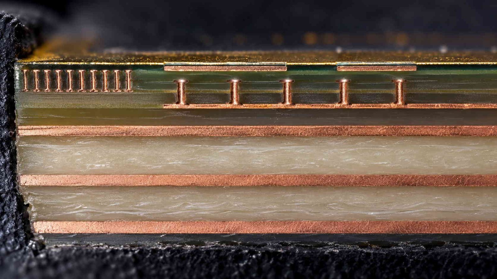
Impedance on a backplane layer is a stackup question with a non-obvious answer. On thin RF cores the dielectric height dominates; on the 0.51 mm stripline geometry of section 2, the ordering inverts and the etch tolerance becomes the largest term — which changes what belongs on the fabrication drawing and what the coupon has to prove.
| Tolerance | ΔZ0 | Change | Where it comes from |
|---|---|---|---|
| Etch, ±5 µm on w = 0.153 mm | ±1.13 Ω | ±2.3 % | Imaging and etch compensation |
| Plane spacing, ±5 µm on b = 0.51 mm | ±0.34 Ω | ±0.7 % | Laminate and lamination tolerance |
| Dk, ±0.02 lot tolerance | ±0.17 Ω | ±0.3 % | Material lot |
| All three adverse at once | +1.6 Ω | +3.3 % | 51.6 Ω against a 50 Ω target |
Computed for the 50 Ω stripline of table 2. The ordering is the opposite of the thin-core D-band case and worth reading twice: on a 0.51 mm plane spacing, etch tolerance dominates and the dielectric height is forgiving. Which tolerance owns the impedance window is a stackup question, so the RF layers of a backplane need their own sensitivity pass, not an inherited rule from either the thin-core or the thick-core world. The general method is in our controlled impedance RF PCB guide.
The worst-case stack lands 3.3 % high before any reflection budget is discussed, and the two largest terms are both fabrication tolerances — image and etch on the width, lamination on the spacing — while the material lot is a rounding error. The response is the same purchasing move as everywhere else in RF fabrication, sized to this stackup: the etch compensation comes from a coupon built on the same panel, the impedance acceptance lives on a TDR coupon, and the drawing names the tolerance that actually owns the window instead of inheriting one. The general rules are in our controlled impedance RF PCB guide.
7. What a Fab Can and Cannot Verify
Every number above resolves to a measurement, and the useful question at backplane scale is where the fabricator's evidence ends and the system integrator's fixture begins. The table draws that line the way a production lot actually supports it.
| Quantity | Where it is measured | What it can and cannot tell you |
|---|---|---|
| Impedance | TDR on a dedicated coupon | Reliable. Same stackup, same panel. |
| Backdrill depth | Microsection / x-ray per panel | The only honest evidence a stub is really gone. |
| Loss trend with frequency | VNA on a coupon, to 67/110 GHz with extenders | Trend and level per centimetre; fixture extraction grows with frequency. |
| Dk on the actual lot | Coupon resonator or ring | The number the design should have used. |
| Skew on a differential pair | Differential TDR on a coupon | Pair-level skew and length-matching verification. |
| Full 1-metre channel S-parameters | System integrator fixture | Not a fab measurement: connectors, cables and calibration dominate. |
The boundary a fabrication line can stand behind at backplane scale: impedance, backdrill depth, coupon loss trend, lot Dk and pair skew are coupon or panel measurements that ship with the lot. A one-metre channel measurement belongs to the system fixture — every dB of it is shared with the connector, the cable and the calibration. A supplier who states that boundary precisely is easier to build a backplane program with than one who quotes the last row. The VNA method is treated in our mmWave PCB VNA testing guide.
The coupon set has to be designed into the panel before the build — TDR structures, a loss-trend line, a Dk resonator and a differential skew pair on the same stackup and the same material lot — and their geometry is its own small discipline. The measurement method for millimetre-wave-scale coupons is set out in the mmWave PCB VNA testing guide, and the inspection regime that backs them — microsection, x-ray, lot traceability — in the RF PCB quality control inspection guide. Definitions for every term on this page are in the high frequency PCB glossary.
8. The DFM Checklist Before Gerber Release
Nothing here is exotic; every item is a line on a drawing or a purchase order, and each traces to a number computed above. The checklist is short on purpose — the expensive failures on metre-scale boards come from ordinary items nobody escalated.
| # | Drawing or PO line item | Why it is on the list |
|---|---|---|
| 1 | Backdrill residual stub ≤ 0.77 mm on RF paths (56 GHz margin) | Stub resonance arithmetic (section 4) |
| 2 | Backdrill depth verified by microsection or x-ray, per panel | Depth control is the deliverable (section 7) |
| 3 | Etch compensation per coupon — etch owns the impedance window | ±5 µm on width is ±2.3 % (section 6) |
| 4 | Line width / plane spacing fixed by stackup, not left to default | Doubling w halves the conductor row (section 2) |
| 5 | Aspect ratio reviewed against plating capability for 4.8–6.4 mm stacks | 19–26:1 needs a plating answer (section 1) |
| 6 | Connector-field xy growth budget: 1.02 mm per metre at ΔT 60 °C | Thermal growth is a millimetre-scale term (section 3) |
| 7 | Pair-skew drawing tolerance in mm, converted from the ps budget | ±1 ps = 0.17 mm of track (section 5) |
| 8 | TDR, loss-trend, Dk and skew coupons on the same lot | The four measurements that back sections 2–7 |
Eight lines, each tracing to a number computed above, all of them cheap on a purchase order and expensive to reconstruct after a first article fails. Items 1–3 decide whether the channel works at all; 4–7 are where the loss and timing budgets are actually spent; 8 is what makes the delivery auditable.
Three questions close the review. Is the backdrill residual stub a specified, microsection-verified dimension — or a process assumption? Does the drawing carry the tolerance that actually owns the impedance window on this stackup — etch, not habit? And does the mechanical drawing spend the 1.02 mm of xy growth explicitly, in the mounting scheme and connector field, instead of leaving it for system integration to discover? A board that answers those three enters fabrication with its loss, timing and alignment budgets under contract.
When the design is earlier than a checklist — choosing between laminate families, or deciding where the hybrid boundary sits — the PCB material comparison chart and our RF PCB manufacturer overview are the right starting points.
PTFE Backplane PCB — Frequently Asked Questions
Why metre-scale midplanes need PTFE-class laminates, how thick they can go, backdrill arithmetic, thermal growth, and what a lot should ship with.
Why does a 1-metre backplane need a PTFE-class laminate at all?
Follow the arithmetic, not the fashion. Over one metre, the dielectric term alone at the 112G Nyquist is 5.7 dB on a Df 0.0013 PTFE-class laminate, 17.6 dB on a Df 0.0037 hydrocarbon, and 106 dB on FR-4. Since a channel budget of a few dB per metre is already being shared with connectors and vias, the dielectric class decides whether a one-metre midplane channel exists at all. The laminate does not, however, fix the channel by itself — on a 0.51 mm stripline geometry the copper owns roughly nine tenths of the nominal budget, which is why line width and stackup appear in the same conversation as Df.
How thick can a PTFE backplane be before manufacturing becomes the problem?
Thickness arrives with layer count: a 24-layer stack averages about 3.2 mm, a 72-layer stack about 6.4 mm. Each step raises the plated aspect ratio — 12.8:1 at 3.2 mm with a 0.25 mm drill, 25.6:1 at 6.4 mm — where hole preparation, desmear and plating chemistry become the limit rather than drilling itself. Every additional millimetre of thickness also deepens the via stub, so the backdrill specification and the plating capability have to be reviewed together, in the same stackup review, before the layout is frozen.
Is backdrilling really mandatory on these boards?
On any RF path through a board thicker than about 1.5 mm, yes, and the number explains itself: an un-backdrilled through via on a 3.2 mm board is a stub resonating at 13.5 GHz on a PTFE-class laminate — roughly half the 28 GHz Nyquist of a 112G-PAM4 channel. To clear the Nyquist the residual stub must stay under about 1.55 mm, and under 0.77 mm to clear 56 GHz. Backdrill depth is therefore a specified, measured dimension — verified by microsection or x-ray per panel — not a process good intention.
What does thermal expansion do to a metre-scale board?
It moves the connector field. At 17 ppm/°C in-plane, a one-metre PTFE-class panel grows about 1.02 mm across a 60 °C swing from assembly to operation, and that growth has to be absorbed in the mounting scheme and connector tolerance stack — a millimetre-scale term, not a rounding error. Through the board thickness the same material grows only a few microns on a 3.2 mm stack, so the z-axis is benign; the warpage and alignment budget is spent in-plane, and it belongs in the mechanical drawing.
What should a PTFE backplane supplier deliver with a lot?
Four coupons and a statement of limits. The coupons: TDR impedance on the production stackup, a loss trend to at least 67 GHz, a Dk measurement on the actual lot, and differential-TDR skew on a representative pair — plus microsection evidence that backdrill depth landed inside specification. The statement: which quantities the fab controls and which belong to the system fixture, where a one-metre channel measurement is dominated by connectors and calibration. A supplier who draws that line precisely is a partner; one who quotes the full channel as a standard deliverable is quoting something their process does not control.
Building a metre-scale PTFE backplane or midplane?
Send us the layer count, the stackup and the connector-field outline. We will review the backdrill specification, the aspect ratio against plating capability, the etch-compensation plan and the xy growth budget before the layout is frozen, and quote fabrication with TDR, loss-trend, Dk and skew coupons from the same lot.
Contact Us → WhatsApp: +86 137 6047 3650Request a PCB Quote
Upload your Gerber ZIP file and project requirements. Our engineering team will review your PCB material, stackup, impedance needs, surface finish, and production quantity before quoting.
Please prepare:
- Gerber files in ZIP format
- PCB material or stackup requirements
- Controlled impedance notes if available
- Prototype or batch production quantity