
Direct Sampling Receiver PCB: Designing the ADC Front End for Low Even-Order Distortion
Direct sampling receiver PCB guide: aperture jitter budgets, differential skew, even-order distortion control, ADC front-end layout, grounding, fab coupons.
Home » ADC Front End » Direct Sampling Receiver PCB: Designing the ADC Front End for Low Even-Order Distortion
Table of Contents
Direct sampling — connecting the antenna-side band to the converter without a mixer stage — is no longer a laboratory architecture. Wideband ADCs now reach first and second Nyquist zones directly, and at European Microwave Week 2026 the component side caught up: amplifier parts aimed explicitly at direct-sampling receivers, with reported even-order output interception around 76 dBm against roughly 36 dBm for a conventional high-linearity driver. The components are ready. The board between them decides how much of that performance survives.
That decision is computable, and this page computes it: what a direct-sampling band plan demands from the front-end filter, the aperture-jitter ceiling the sampling clock sets, how much even-order cancellation a differential channel actually preserves as a function of its own imbalance, what a picosecond of skew is worth in millimetres and degrees, where a bandpass-sampled fold lands, and why an un-backdrilled via matters on a board whose signal band is only a few gigahertz. Every figure is computed; the assumptions are stated where they are used.
The architecture-level comparison — when to sample directly, when to keep a mixer, filter planning and gain distribution — is treated in our EW PCB wideband design guide, and the software-defined variant in the space-grade SDR PCB guide. This page is about the one component direct sampling makes non-negotiable: the ADC front-end board.
1. What Direct Sampling Removes — and Hands to the Board
A mixer stage used to absorb the hard problems: image rejection, out-of-band spurious, wideband gain. Remove it and every one of those jobs moves onto the PCB in analog form, before the converter. The table shows the planning for a representative 5 GS/s sampler.
| Input band of interest (Fs = 5 GS/s) | Nyquist zone used | Where it lands after sampling | Front-end filter consequence |
|---|---|---|---|
| 0.5–2.5 GHz (L/S EW bands) | NZ1, upright | 0.5–2.5 GHz | Anti-alias needed only above 2.5 GHz |
| 2.5–5.0 GHz (S/C) | NZ2, mirrored | folds to 2.5–0 GHz | Passband flat and matched to 5 GHz; jitter budget rises with fin |
| 5.0–7.5 GHz (C) | NZ3, upright | folds to 0–2.5 GHz | Reject both below 5 and above 7.5 GHz; loss budget reaches 7.5 GHz |
| 4.0–6.0 GHz (straddles NZ2/3) | Seam at 5 GHz | folds to 1–0–1 GHz | Unusable without digital correction — move the seam out of band |
Nyquist planning for a representative 5 GS/s converter; the same arithmetic applies at any Fs. Direct sampling trades a mixer stage for filter complexity, and both of those live on the PCB: the anti-alias/-band-select filter corners, the flatness of the front end all the way to the highest sampled frequency, and the loss budget that reaches two to three times the nominal signal band. The last row is the trap: an input band that straddles a zone boundary folds onto itself at DC-class frequencies, and no filter fixes a seam inside the band. Band planning of the conventional superheterodyne alternative is treated in our EW PCB wideband design guide.
The pattern across the rows: as the sampled band moves up, the front-end filter gains corners on both sides, the insertion-loss budget stretches to two or three times the nominal signal band, and out-of-band content — anywhere that folds into the digitised band — becomes an in-band threat. The board-level loss and matching work behind those budgets is the same 50-ohm discipline set out in our 50 ohm RF trace guide; the filter corners themselves are a system decision that belongs on the fabrication drawing, not in a module datasheet.
2. The Sampling Clock Is the First Component: the Jitter Ceiling
Before any noise figure or filter loss, one number caps a direct-sampling receiver: the aperture jitter of the clock that strokes the converter. The ceiling is pure arithmetic.
| Clock aperture jitter tj | SNR ceiling @ 100 MHz | @ 1 GHz | @ 5 GHz | Verdict for a 5 GHz-input sampler |
|---|---|---|---|---|
| 10 ps (catalog crystal XO) | 44.0 dB | 24.0 dB | 10.1 dB | Unusable at any wideband input |
| 1 ps (good dedicated clock) | 64.0 dB | 44.0 dB | 30.1 dB | Marginal — the clock, not the ADC, sets the noise floor |
| 250 fs (RF-grade clock + filtering) | 76.1 dB | 56.1 dB | 42.1 dB | Workable for wideband EW capture |
| 100 fs (reference-grade distribution) | 84.0 dB | 64.0 dB | 50.1 dB | Clean — board choice (stub-free path, solid return) starts to matter more than the oscillator |
SNR = −20·log10(2π·f_in·t_j) — the aperture-jitter ceiling, before converter noise, before board losses. Two consequences follow. First, the sampling clock is the first component in the receiver: a 10 ps catalog oscillator caps a 5 GHz input at 10 dB SNR no matter how good the ADC is. Second, at reference-grade jitter the board takes over: any unplanned stub, split return path or ringing edge on the clock line adds its own timing noise, so the clock distribution is routed like an RF path — which is the standard we apply on our controlled impedance RF PCB builds.
Read the table twice. First as a component decision: the gap between a 10 ps catalog oscillator and a 100 fs distribution is 40 dB of SNR at a 5 GHz input — no ADC choice recovers it. Then as a board decision: once the clock is reference-grade, the remaining timing noise comes from the board itself — ringing edges, stub resonance on the clock line, a return path that detours. That is why the clock distribution on a direct-sampling receiver is routed with RF rules end to end, and why the launch into the clock pin gets the same treatment as any antenna feed — the geometry discipline is in our RF connector launch guide.
3. Even-Order Distortion: Where 40 dB of Device Improvement Is Won or Lost
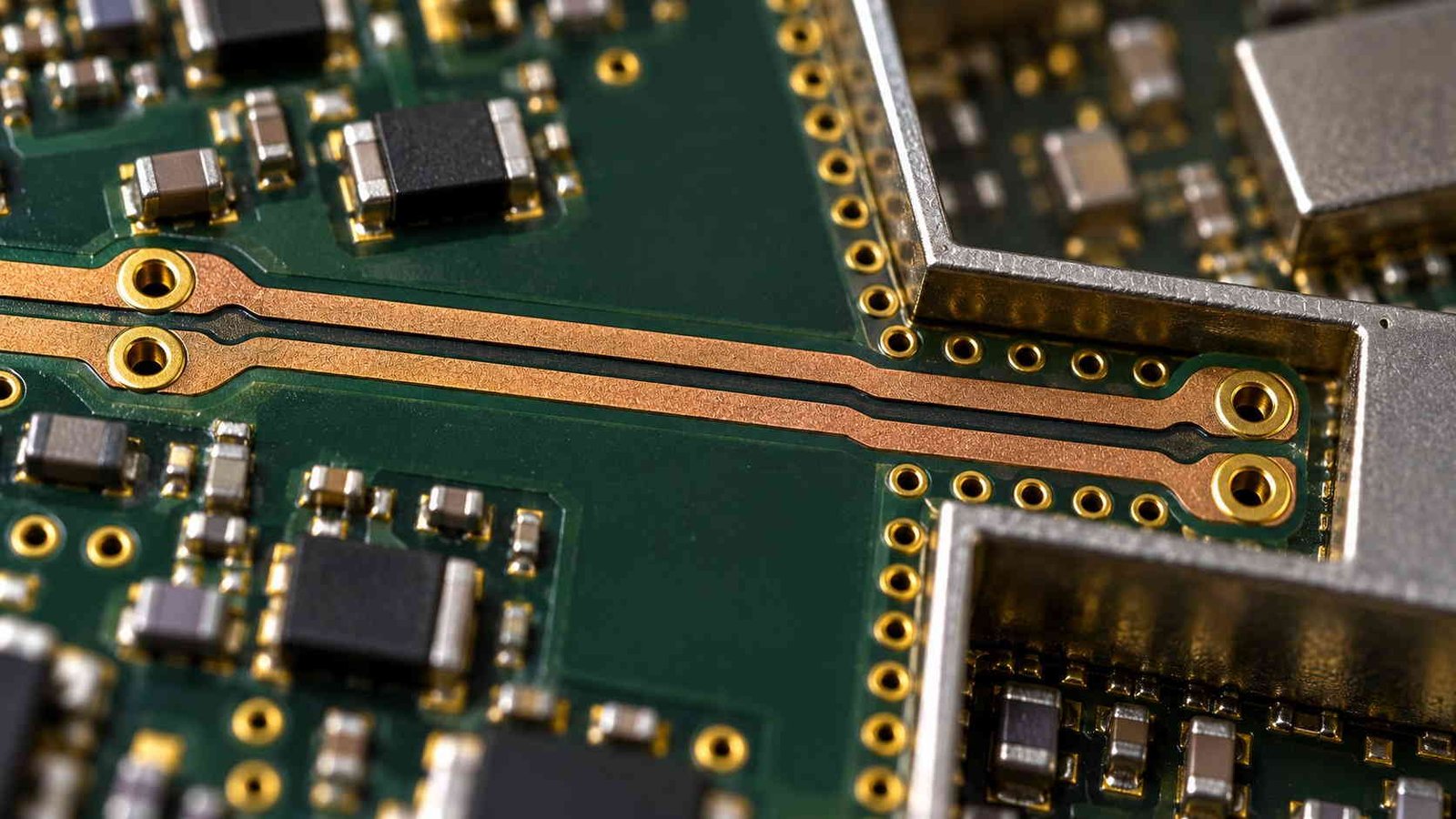
Even-order products are the signature distortion of a direct-sampling chain, and the newest amplifier generation attacks them head-on: the reported EuMW 2026 comparison put a suppression-type part at OIP2 ≈ 76 dBm against ≈ 36 dBm for a conventional driver — about 40 dB more headroom, shipping now. The device assumes one thing: that the two branches it drives are mirror images. The table prices what happens when the board’s differential channel is not.
| Amplitude imbalance | Phase imbalance | Residual even-order suppression | What it does to the chain |
|---|---|---|---|
| ±0.1 dB | ±1° | 33.5 dB | Device-class suppression survives the board |
| ±0.1 dB | ±5° | 21.1 dB | Most of a 40 dB device advantage is gone |
| ±0.5 dB | ±1° | 24.2 dB | Amplitude symmetry alone is not enough |
| ±0.5 dB | ±5° | 19.4 dB | Suppression capped around 20 dB |
| ±1.0 dB | ±5° | 16.3 dB | Worse than many stages’ own IM2 — the board is now the dominant distortion source |
Residual = 20·log10|r·e^{jθ} − 1| for two mirrored branches with amplitude ratio r and phase error θ. The context is the amplifier generation shown at EuMW 2026 aimed at direct-sampling receivers, where reported demonstration conditions compared a conventional high-linearity driver at OIP2 ≈ 36 dBm with a suppression-type part at ≈ 76 dBm — an improvement of about 40 dB, in a device that is shipping now. The table is the board-side mirror of that number: a differential channel that only cancels to 21 dB delivers four-fifths of the device’s advantage to the scrapyard, and no later DSP stage can recover a folded second-order product that lands in-band. Symmetry of the differential structure — mirrored pads, anti-pads, via transitions, no single-ended stubs inside the pair — is what keeps θ small, and the grounding that keeps the branches identical is the same mixed-signal discipline set out in our mixed-signal high-speed design overview.
The verdict column is the argument for board-level symmetry discipline. ±0.1 dB and 1° preserves the device-class result; the imbalances that creep in with asymmetric vias, an unmirrored layer transition or a return-plane split burn the 40 dB down to under 20 — and the residual second-order product is not background noise, it is a discrete tone at 2f that folds in-band and stays. This is also why a high-OIP2 part cannot be evaluated on a board with unknown symmetry: the measurement would report the board, not the device. The grounding and partitioning that keep both branches identical are treated in our mixed-signal high-speed design overview.
4. Skew Is a Dimension: What a Picosecond Is Worth
Differential skew is usually discussed as a digital timing parameter. In a direct-sampling receiver it is the second-order distortion parameter, because the IM2 product forms at the second harmonic — where every picosecond counts double in degrees.
| Intra-pair skew Δt (stripline, εr,eff 3.0) | Length equivalent | Phase error at 2f = 2 GHz | Phase error at 2f = 5 GHz |
|---|---|---|---|
| 0.5 ps | 0.09 mm | 0.36° | 0.90° |
| 1.0 ps | 0.17 mm | 0.72° | 1.80° |
| 2.0 ps | 0.35 mm | 1.44° | 3.60° |
| 5.0 ps | 0.87 mm | 3.60° | 9.00° — the suppression spec is dead |
Skew converts to length at v = c/√εr,eff (0.173 mm/ps on εr,eff 3.0) and to phase at the second harmonic: the IM2 product at 2f sees twice the phase error of the fundamental, so 5 ps is 9° exactly where the even-order cancellation happens. Working backwards, holding phase imbalance to 1° at 2f = 5 GHz (a 2.5 GHz input) allows 0.56 ps ≈ 0.10 mm of skew — which is why intra-pair length matching on a direct-sampling receiver is specified at ±0.10 mm, coupon-verified, not eyeballed in CAD. The propagation model behind the numbers is the microstrip/stripline treatment in our microstrip vs stripline guide, and the matching discipline is part of the controlled impedance RF PCB method.
The working number falls out of the last row: to hold phase imbalance near 1° at 2f = 5 GHz, intra-pair skew must stay under about 0.6 ps — one tenth of a millimetre of matched length. That is a fabrication dimension with a coupon measurement attached, and it is why the matching on these boards is specified and verified rather than assumed. Note what the table also says: amplitude symmetry alone (the ±0.5 dB, 1° row of the previous table) does worse than tight phase matching — the geometry is the larger term.
5. Bandpass Sampling and the Fold: Filter Consequences on the Board
Direct sampling does not always mean sampling the first Nyquist zone. Bandpass sampling lets a 5 GS/s converter digitise a 5–7.5 GHz band directly — trading a mixer for filter complexity that lands entirely on the board.
| Front-end plan (Fs = 5 GS/s) | Folded position | What the board must do |
|---|---|---|
| Sample NZ1 directly: 0.5–2.5 GHz | Upright, 0.5–2.5 GHz | Anti-alias above 2.5 GHz only; simplest filter, lowest loss budget |
| Bandpass-sample NZ2: 2.5–5.0 GHz | Mirrored to 2.5–0 GHz | Front end stays flat and matched to 5.0 GHz; out-of-band spurs fold into the digitised band |
| Bandpass-sample NZ3: 5.0–7.5 GHz | Upright, 0–2.5 GHz | Reject both below 5 and above 7.5 GHz; insertion-loss budget now reaches 7.5 GHz |
| Band 4.0–6.0 GHz across the seam | Folds onto itself: 1–0–1 GHz | No filter can repair a seam inside the band — the Fs choice is a front-end decision |
Bandpass (harmonic) sampling is how a direct-sampling receiver covers C-band without a 10 GS/s converter — but the fold is an electrical fact the front end has to respect: content from any other Nyquist zone lands in the digitised band, so the anti-alias filter’s rejection is specified against all frequencies that map to it, not just the adjacent band. On the PCB that means the passband flatness and match extend to the highest sampled frequency, the filter skirt is a system requirement on the drawing, and the sampling-clock spurious content is treated as an in-band threat. The wideband filter-and-gain planning side is treated in our EW PCB wideband design guide.
The last row is the one that ends design reviews early: a band chosen across a zone boundary folds onto itself, and nothing downstream corrects it. Everything else on the table is manageable but explicit — rejection specified against all folding frequencies, flatness and match extended to the highest sampled edge, clock spurious treated as in-band. A fabricator who asks for the Nyquist plan at RFQ is not being curious; the fold decides where the loss budget and the filter corners go, which decides the stackup.
6. Via Stubs: Why They Matter on a Board Whose Band Is “Only” a Few GHz
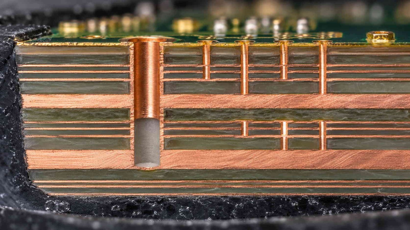
The signal band of a 5 GS/s receiver tops out near 2.5–3 GHz — comfortably below the frequencies where fabricators reflexively backdrill. The input path and the clock path disagree with that reflex, for two reasons: second-order content lives at 2f, and the sampling clock is a square wave whose harmonic series runs past 10 GHz. The stub arithmetic:
| Residual stub on input or clock path (εr 3.48) | First λ/4 resonance | Verdict for a direct-sampling receiver |
|---|---|---|
| 0.5 mm (backdrilled) | 80.4 GHz | Clear of the band, of 2f content and of clock harmonics |
| 1.0 mm | 40.2 GHz | Acceptable ceiling for RF paths |
| 1.6 mm un-backdrilled through via (1.6 mm board) | 25.1 GHz | Above the band — but inside the harmonic content of a 2.5–3 GHz sampling clock |
| 2.4 mm un-backdrilled through via (2.4 mm board) | 16.7 GHz | Sits on the sampling clock’s harmonic series — edge ringing and timing noise couple straight in |
f = c/(4·L·√εr). A direct-sampling input path carries more than the signal band: second-order products live at 2f, and the sampling clock is a square wave whose harmonic series extends past 10 GHz — so a stub resonance anywhere in the 12–30 GHz region is not harmless just because it sits above the signal band. On a 2.4 mm board every un-backdrilled through via on the input or clock path resonates at 16.7 GHz, square in the clock’s harmonics; holding the residual stub to ≤ 1.0 mm puts the first resonance at 40 GHz and out of the way. Backdrill depth is verified by microsection or x-ray per panel — the method and tolerances are in our back drill PCB guide and drilling capabilities page.
A 2.4 mm board with un-backdrilled through vias puts a 16.7 GHz resonance on every input and clock path — square in the clock’s harmonic series, where a resonance converts edge ringing into timing noise and couples it straight into the conversion. Holding the residual stub to ≤ 1.0 mm lifts the first resonance to 40 GHz, out of every mechanism this architecture has. The verification is dimensional, not procedural: microsection or x-ray per panel, to the tolerances in our back-drill guide.
7. The Low-Even-Order-Distortion Fabrication Package
A direct-sampling receiver board is bought on symmetry, and symmetry is a measurable deliverable. The package below turns the numbers of sections 2–6 into drawing lines and coupon reports.
| # | Drawing or PO line item | Why it is on the list |
|---|---|---|
| 1 | Intra-pair skew ≤ 0.10 mm (0.58 ps) on ADC inputs, coupon-verified | 0.96° at 2f = 5 GHz — the IM2 budget (section 4) |
| 2 | Mirrored differential structure: symmetric pads, anti-pads, vias; no single-ended stubs inside the pair | Phase imbalance is the larger cancellation term (section 3) |
| 3 | Unbroken return plane under the whole differential path and the clock line | Any split forces one branch around and unbalances the pair (section 3) |
| 4 | Clock path routed as RF: residual stub ≤ 1.0 mm, guard ground vias, dedicated low-noise clock | Jitter ceiling and clock harmonics (sections 2, 6) |
| 5 | Analog/digital supplies isolated; PDN filtering on the drawing | Even-order products convert supply noise into in-band spurs (section 3) |
| 6 | Low-PIM surface finish on RF pads (immersion silver or bare copper preferred) | ENIG’s nickel layer is ferromagnetic — a passive-IM2 risk on high-OIP2 front ends (section 7) |
| 7 | Differential TDR + loss-trend coupons: impedance, skew, insertion loss to 2f | Skew and loss verified by measurement, not asserted from CAD (section 4) |
| 8 | IPC Class 3 + microsection/x-ray evidence package per panel | Backdrill depth, plating and registration auditable (section 6) |
Eight lines, each tracing to a number computed above. Items 1–3 are where the even-order distortion budget is won or lost; 4–5 keep the clock and supplies from re-injecting what the symmetry removed; 6–8 are what make the result measurable and auditable. A receiver board that ships with these eight answered lets the high-OIP2 devices around it do their job.
One item deserves its own paragraph: surface finish. The nickel in ENIG is ferromagnetic, and ferromagnetic metallisation under strong RF fields is a recognised passive intermodulation mechanism — on a board built around 76 dBm-class even-order suppression, a PIM-prone finish on the RF pads works directly against the devices it connects. Immersion silver or bare copper on RF pads, with the finish choice documented at stackup review, keeps the finish from becoming the distortion budget’s hidden term.
For the adjacent decisions — reading a datasheet before committing a laminate to the panel, or qualifying the finished board — the PCB material comparison chart, the mmWave PCB VNA testing guide, the quality control and inspection overview and our RF PCB manufacturer page are the right starting points.
Direct Sampling Receiver PCB — Frequently Asked Questions
What direct sampling hands to the board, the jitter ceiling, even-order cancellation arithmetic, how tight skew must be, surface finish, and what the fab package should ship with.
What does direct sampling change on the PCB itself?
It removes mixer stages and hands their jobs to the board. The front-end filter must now reject every frequency that folds into the digitised band, the passband must stay flat and matched to the highest sampled frequency (which can be two to three times the nominal signal band), the sampling clock is routed as an RF path because its jitter sets the noise floor, and the differential connection to the ADC has to be symmetric enough to preserve the device-level even-order distortion suppression. Direct sampling is architecturally simpler and electrically stricter — the board carries the difference.
Why doesn’t a high-OIP2 amplifier fix board-level even-order distortion?
Because the amplifier’s suppression works on the pair of mirrored signals it sees, and the board is what makes them mirrored. A differential channel with ±0.5 dB and 5° of imbalance cancels second-order products to only about 19 dB — so of the roughly 40 dB improvement a suppression-type device adds over a conventional driver (reported at EuMW 2026: OIP2 ≈ 76 dBm vs ≈ 36 dBm in demonstration conditions), most is thrown away before the ADC. Worse, the residual product is a real signal at 2f that folds in-band; no DSP stage can remove it later. The fix is board symmetry: mirrored geometry, matched length to about ±0.10 mm, and an unbroken return plane.
How tight does differential matching actually have to be?
Tighter than most digital rules, because the phase error counts at the second harmonic. On a stripline layer with εr,eff 3.0, 1 ps of skew is 0.17 mm of length and 1.8° of phase error at 2f = 5 GHz. Holding phase imbalance near 1° where the IM2 product forms allows about 0.56 ps — roughly 0.10 mm of intra-pair skew. That is a coupon-verified fabrication dimension, not a CAD-side nicety, and layer transitions, pad stacks and any series elements must be mirrored so the two branches stay electrically identical.
Which surface finish should a low-distortion receiver board use?
On the RF pads, a low-passive-IM2 finish: immersion silver or bare copper (with plating chosen for solderability elsewhere). ENIG deposits a nickel layer, and nickel is ferromagnetic — under the strong local fields of a wideband front end it is a recognised passive intermodulation risk, which is exactly the distortion mechanism a high-OIP2 direct-sampling receiver exists to avoid. Where ENIG is required for assembly reasons, keeping it off the RF signal pads and documenting the exception is the compromise; the choice belongs in the stackup review, not as a default.
What should a low-even-order-distortion fabrication package include?
The measurements that prove the symmetry budget: differential TDR impedance on both branches, intra-pair skew on the production panel, insertion loss to 2f from a loss-trend coupon, microsection or x-ray evidence that clock-path backdrill depth landed inside specification, all to IPC Class 3. Add the material data that lets the customer simulate the channel — Dk/Df versus frequency, copper roughness — and the package turns the board from a passive part into a dataset the receiver team can correlate against its own two-tone tests. The measurement method is set out in our RF/mmWave test fixture and VNA testing guides.
Building a direct-sampling receiver or wideband ADC front-end board?
Send us the input band, sample rate and ADC pinout. We will review the Nyquist plan against your front-end filter, the differential skew and symmetry budget, the clock path and surface finish at stackup review, and quote fabrication with differential TDR, skew and loss-trend coupons plus an IPC Class 3 evidence package.
Contact Us → WhatsApp: +86 137 6047 3650Request a PCB Quote
Upload your Gerber ZIP file and project requirements. Our engineering team will review your PCB material, stackup, impedance needs, surface finish, and production quantity before quoting.
Please prepare:
- Gerber files in ZIP format
- PCB material or stackup requirements
- Controlled impedance notes if available
- Prototype or batch production quantity