
Space-Grade SDR PCB: Wideband Front End, Converter Interface and Vacuum-Compatible Stackup
Space-grade SDR board design: a wideband RF front end, a multi-gigabit converter interface and a vacuum environment on one stackup.
Home » High Frequency PCB » Space-Grade SDR PCB: Wideband Front End, Converter Interface and Vacuum-Compatible Stackup
Table of Contents
A software-defined radio is a converter with analog built around it. That one sentence explains most of the layout decisions on the board: the aperture feeds a low-noise amplifier, a switched filter bank, a mixer and an ADC; the FPGA does the rest; on transmit the chain runs the other way through a DAC and a power amplifier. Everything that is hard about the board sits at the boundaries between those three domains — RF, converter, digital — because each one wants a different reference plane, a different stackup and a different definition of "matched".
The procurement trend behind this class of board is toward smaller terminals with wider instantaneous bandwidth, built on a software-defined platform and intended for production rather than a single demonstration unit. That combination puts three constraints on the same piece of laminate: the front end has to work over several octaves instead of a tuned band, the converter interface has to run at multi-gigabit lane rates, and the assembly has to survive an environment where there is no air to carry heat away. None of those is new individually. What is new is that they are now on one board, at one thickness, in one reflow cycle.
The numbers in this guide come from a single set of models, stated once here so they can be checked: 50 Ω microstrip on 0.508 mm dielectric, 1 oz copper, roughness multiplier 1.8, dielectric and conductor loss computed separately. At 6 GHz, 100 mm of 50 Ω line costs 0.47 dB on a low-loss PTFE-class laminate, 0.79 dB on a hydrocarbon and 2.61 dB on FR-4. A 12-bit converter has a 74 dB quantization limit, and 100 fs of clock jitter at 6 GHz leaves you 7.8 effective bits. Those two numbers — loss and jitter — decide whether the board works; everything else is detail around them.
Stackup partitioning for mixed RF and digital boards is covered in our RF and digital mixed-signal stackup guide, the manufacturing side of the same problem in RF PCB manufacturing for mixed-signal designs, and the material families — parameter by parameter — in the high frequency PCB materials section. This page connects them: what the numbers have to be on a wideband SDR board, and where each one is decided.
1. What the Board Has to Do, and Why SDR Boards Fail at the Seams
Start with the dynamic range, because it explains why a wideband front end is a different design problem from a tuned one. A receiver with 1 GHz of instantaneous bandwidth has a thermal noise floor of −84 dBm; with a 3 dB noise figure it is −81 dBm. A converter with a 2 Vpp differential full scale presents +10 dBm at its input. The distance between those two numbers is 91 dB, and that is the entire analog range the board has to preserve.
Now change the bandwidth. At 500 MHz the floor drops to −84 dBm and the range grows to 94 dB; at 100 MHz it is 101 dB. Every factor of ten in bandwidth costs 10 dB of range, and there is no architecture that avoids it — the noise is in the band, not in the part. This is the first reason an SDR board is harder than a single-band radio: it is asked to deliver the dynamic range of a narrowband receiver while listening to ten narrowband receivers at once.
| Instantaneous bandwidth | kTB noise floor | With 3 dB NF | Converter full scale | Digital range | SFDR at IIP3 +10 dBm |
|---|---|---|---|---|---|
| 100 MHz | −94.0 dBm | −91.0 dBm | +10 dBm (2 Vpp diff) | 101 dB | 60.7 dB |
| 500 MHz | −87.0 dBm | −84.0 dBm | +10 dBm (2 Vpp diff) | 94 dB | 60.7 dB |
| 1 GHz | −84.0 dBm | −81.0 dBm | +10 dBm (2 Vpp diff) | 91 dB | 60.7 dB |
Noise floor is −174 dBm/Hz plus 10·log(bandwidth); SFDR is (2/3)(IIP3 − noise floor) for a third-order-limited front end. A 2 Vpp differential full scale into 50 Ω is +10 dBm. Two things follow: a wideband front end loses 10 dB of range every time the bandwidth goes up by a factor of ten, and the converter is not what limits it — the analog front end and the clock do.
The third column that matters is linearity. With an input intercept point of +10 dBm, the spurious-free dynamic range is 60.7 dB. That number is set by the first amplifier and by the filter ahead of it, not by the converter, and it degrades the moment a strong out-of-band signal reaches the amplifier uncompressed. On a wideband front end there is no narrow filter to remove that signal, which is why the switched filter bank exists and why its loss lands directly in the noise figure.
The seams are where boards actually fail. RF-to-converter: the reference plane changes from a controlled-impedance RF ground to a digital ground, and the transition is a via or a balun. Converter-to-digital: the lane rate is high enough that a stub or a connector pin is a transmission line discontinuity. Digital-to-RF: switching noise from the FPGA finds the front end through the power distribution network, not through the air. Three seams, three different fixes, and a review that treats them as one problem will miss two of them.
2. Partitioning the Stackup: Three Domains, One Laminate Stack
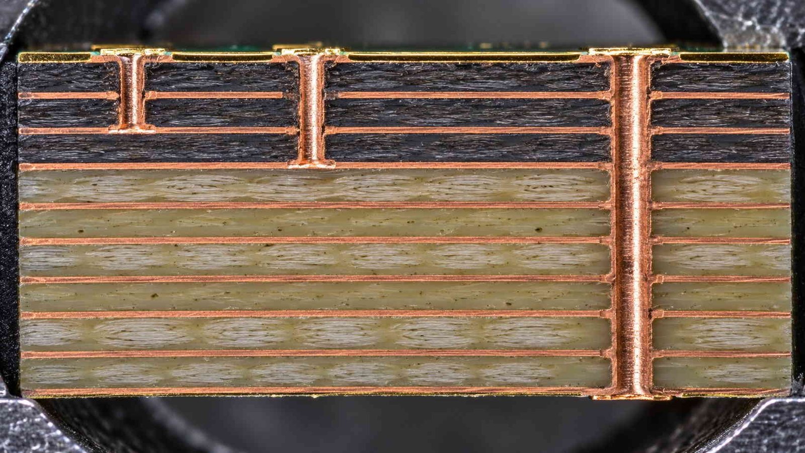
The stackup is where the architecture becomes physical, and the constraint that drives it is not layer count but adjacency. Every signal layer needs a plane next to it, and the plane has to be the one the signal is referenced to — not a plane that happens to be nearby. On a mixed board that rule alone decides most of the layer assignment, because the RF section wants ground, the lane section wants ground, and the only thing that legitimately wants power is the power section.
| Layer | Function | Reference | Material class | Thickness |
|---|---|---|---|---|
| L1 | RF in / out, antenna ports, filter pads | L2 ground | Low-loss laminate | 0.508 mm |
| L2 | Solid ground, no splits | — | Low-loss laminate | 0.508 mm |
| L3 | Feed network, stripline RF | L2 / L4 | Low-loss laminate | 0.254 mm |
| L4 | Ground, shield reference | — | Low-loss laminate | 0.508 mm |
| L5–L6 | Converter lanes (JESD204B/C) | Ground | Low-loss or mid-loss | 2 × 0.1 mm |
| L7–L8 | Digital bus, memory, control | Ground | FR-4 | 2 × 0.1 mm |
| L9–L10 | Power planes, paired and stitched | — | FR-4 | 2 × 0.2 mm |
| L11–L12 | Low-speed control, connectors, thermal spread | Ground | FR-4 | — |
One example 12-layer build, not a template. The point of the table is the reference column: every signal layer sits next to a plane, the RF and converter sections reference ground rather than power, and no RF or lane crosses a plane boundary. The upper four layers are a low-loss laminate, the rest is FR-4, which is the normal hybrid arrangement for this class of board.
Two details in that table are worth pulling out. First, the RF and lane sections do not reference the power planes, even though a plane is a plane electrically: a power plane carries the switching noise of everything it feeds, so a lane referenced to it inherits that noise as common-mode. Second, the transition from low-loss laminate to FR-4 happens at a ground layer, not at a signal layer, so that the material change does not coincide with an impedance change. Both are cheap at the layout stage and expensive afterwards.
The hybrid itself is normal practice and it works, but it moves the failure modes to the interface: registration between the two materials, z-axis CTE difference through any barrel that crosses the boundary, and warp on a large panel. The fabrication side of that is set out in FR4 Rogers hybrid PCB, and the design-side isolation rules for a mixed board in the mixed-signal stackup article. What is specific to a space-bound SDR is that the same interface also has to pass thermal cycling and outgassing, which is covered in section 6.
One number decides how much of the stack can be low-loss: the loss budget. If the front end can spend 0.5 dB on 100 mm of feed, a low-loss laminate buys the whole run; if it can spend 0.5 dB on 300 mm, it buys 150 mm and the rest has to be stripline in FR-4 with the loss accounted for. Deciding that at layer-assignment time is a five-minute calculation; discovering it after the first prototype is a re-spin.
3. The Wideband Front End: Loss Scales with Root Frequency
Wideband front-end loss is not a single number, and budgeting it at midband is the most common mistake on this class of board. Both loss mechanisms scale with frequency: conductor loss with the square root of frequency through skin depth, dielectric loss linearly with frequency through the loss tangent. From 0.5 GHz to 6 GHz that is a factor of 3.5 in dielectric loss and 3.5 in conductor loss, so a link budget written at 2 GHz understates the top of the band by more than 3 dB.
| Laminate class (εr / Df) | 1 GHz | 3 GHz | 6 GHz | 10 GHz | Dielectric share at 6 GHz |
|---|---|---|---|---|---|
| PTFE, low loss (2.20 / 0.0009) | 0.17 dB | 0.32 dB | 0.47 dB | 0.63 dB | 14 % |
| Hydrocarbon (3.48 / 0.0027) | 0.26 dB | 0.51 dB | 0.79 dB | 1.11 dB | 31 % |
| FR-4 (4.30 / 0.0200) | 0.59 dB | 1.44 dB | 2.61 dB | 4.11 dB | 76 % |
50 Ω microstrip, 0.508 mm dielectric, 1 oz copper, roughness multiplier 1.8; values are per 100 mm and are computed from the dielectric and conductor terms, not measured. Use them for comparison and scaling, not as a substitute for a coupon: absolute loss typically lands within 20 % of this model, and the ranking between classes is more reliable than the absolute number.
The column that changes design decisions is the last one. On a 0.508 mm low-loss laminate at 6 GHz, only 14 % of the loss is dielectric — the other 86 % is copper. On that stack, chasing a lower loss tangent buys almost nothing; what buys something is smoother copper foil, a thicker dielectric, or a wider line. On FR-4 the ratio inverts: 76 % of the loss is dielectric, so the material is the lever and the copper is nearly irrelevant. Two boards, same frequency, opposite engineering priorities.
There is a second wideband problem that a loss table does not show. A 0.5–6 GHz front end has to hold 50 Ω across a 12:1 bandwidth, and no single line geometry is optimal over that range. What actually limits the top octave is usually not the line but the transitions: a connector launch that is fine at 2 GHz can have a 5 GHz resonance, and a filter pad designed for a 1.5 GHz part presents a capacitive discontinuity that costs 0.3 dB at 6 GHz. The launch rules are in our RF connector launch guide, and the filter-side layout in the QFN MMIC RF layout article.
Gain slope is the third term and it is not a PCB problem, but it lands on the PCB. A wideband amplifier with 20 dB at 0.5 GHz and 14 dB at 6 GHz has a 6 dB slope across the band, which the equaliser or the digital back end has to remove — and every passive equaliser costs loss and adds a resonance of its own. The reason to know the slope before layout is that it decides where the filter bank sits and how much loss the board can afford between stages. Laminate comparisons at the parameter level are in PTFE materials and Rogers materials; the definitions behind them are in the high frequency PCB glossary.
4. Jitter, ENOB and the Clock That Sets the Dynamic Range
Ask an SDR designer what limits the dynamic range and the answer is usually the converter. Measure the board and the answer is usually the clock. The relationship is unforgiving and simple: SNR from aperture jitter is −20·log10(2π·f·t_rms), so the penalty grows with input frequency and with jitter in the same way. Double the frequency, lose 6 dB. Double the jitter, lose 6 dB.
| Input frequency | 100 fs rms | 200 fs rms | 500 fs rms | 1 ps rms |
|---|---|---|---|---|
| 1 GHz | 10.3 bit | 9.3 bit | 8.0 bit | 7.0 bit |
| 3 GHz | 8.8 bit | 7.8 bit | 6.4 bit | 5.4 bit |
| 6 GHz | 7.8 bit | 6.8 bit | 5.4 bit | 4.4 bit |
Effective number of bits from SNR = −20·log10(2π·f·t_rms), ENOB = (SNR − 1.76)/6.02. A 12-bit converter has a 74.0 dB quantization limit; a 14-bit one has 86.0 dB. At 6 GHz, holding that 12-bit limit would need 5 fs of clock jitter, which does not exist in a real clock tree — so above about 3 GHz the converter resolution is not the number on the datasheet, it is the number the clock allows.
Read the table against the converter datasheet. A 12-bit part specifies 74 dB of quantization SNR; at 6 GHz that would require 5 fs of clock jitter, which no real clock tree delivers. A 100 fs budget gives 7.8 effective bits at 6 GHz and 8.8 at 3 GHz, so the 12-bit converter is behaving like an 8-bit one at the top of the band — and that is the good case, with a well-designed clock. At 500 fs, which is what an ordinary oscillator plus an ordinary buffer plus a switching supply will give you, the same board delivers 5.4 bits.
This is why the clock is a board-level design task and not a component selection. Jitter arrives from four places, and three of them are on the board: the oscillator, the buffer that distributes it, the supply that powers the buffer, and the reference plane the clock trace runs over. A budget looks like the one below — allocations, not measurements, but allocations are how the tree gets designed.
| Contributor | Allocation (rms) | What sets it |
|---|---|---|
| Reference oscillator | 60 fs | Part choice, and whether it is multiplied on board |
| Clock buffer / divider | 40 fs | Additive jitter from the datasheet, at the actual output frequency |
| Supply-induced jitter | 50 fs | LDO instead of a switching rail, and local decoupling at the buffer |
| Board and reference plane | 30 fs | No split crossings, no vias in the clock path, matched lengths |
| Root sum square | 92.7 fs | Lands at 7.9 ENOB at 6 GHz, 8.9 at 3 GHz |
An allocation, not a measurement: allocations are how the clock tree gets designed, and the RSS is what it adds up to. The last row is the one that surprises people — a budget made of four modest numbers still lands just under 100 fs, which is exactly where a 12-bit converter stops being 12 bits above 3 GHz. If the requirement is 10 effective bits at 6 GHz, the oscillator alone has to be better than 50 fs.
The board's own contribution is the one designers most often leave out, because it does not appear in any datasheet. A clock trace that crosses a plane split detours its return current, and the detour adds both delay and jitter; a clock buffer powered from the same switching rail as the FPGA inherits that ripple as phase modulation; a via in the clock path is a stub that shows up as a few hundred femtoseconds at 6 GHz. The rules follow directly: clock on its own layer with a continuous ground, no vias if the geometry allows, a linear regulator for the buffer, and physical separation from the switching supplies. The grounding and shielding principles are the same ones set out in the LNA grounding and shielding guide, applied to a digital signal instead of an analog one.
5. The Converter Interface: 12.5 Gbps Lanes and a 16 ps Budget
The converter interface is where the board stops being an RF board and becomes a high-speed digital board, and the currency changes with it. RF matching is measured in degrees; lane matching is measured in picoseconds, and picoseconds are much smaller. At 12.5 Gbps the unit interval is 80 ps, a workable skew budget is 0.2 UI or 16 ps, and at 5.52 ps per millimetre in hydrocarbon laminate that is 2.9 mm of length mismatch. Three millimetres — a routing detour around a connector — consumes the entire budget.
| Lane rate | Unit interval | 0.2 UI budget | In laminate (5.52 ps/mm) | In FR-4 (6.03 ps/mm) |
|---|---|---|---|---|
| 6.25 Gbps | 160 ps | 32.0 ps | 5.8 mm | 5.3 mm |
| 12.5 Gbps | 80 ps | 16.0 ps | 2.9 mm | 2.7 mm |
| 15.5 Gbps | 64.5 ps | 12.9 ps | 2.3 mm | 2.1 mm |
Converter lanes are matched in time, and time is a much harsher currency than phase. A 3 mm mismatch that would be tolerable on a 1.5 GHz RF feed is a third of the entire skew budget at 12.5 Gbps. The two right-hand columns also show why a lane should stay in one dielectric: the same 100 mm of trace is 552 ps in hydrocarbon and 603 ps in FR-4, so 20 mm of material change moves the lane by about 10 ps without any layout change at all.
The right-hand columns explain a rule that hybrid stackups break without anyone noticing. The same 100 mm of trace is 552 ps in hydrocarbon and 603 ps in FR-4, a difference of 0.51 ps per millimetre. If four lanes of a converter pair run 20 mm on one material and 20 mm on the other — because the bus crosses from the low-loss section into the FR-4 section — they arrive about 10 ps apart before any routing error is counted. On a 12.5 Gbps link that is more than half the budget, produced by the stackup rather than by the layout. Keep a lane in one dielectric, or match the crossing on all lanes symmetrically.
Three further rules decide whether the link closes. Each differential pair is matched intra-pair to a small fraction of a UI, because intra-pair skew turns directly into common-mode conversion and eye closure. Every lane in a group has the same number of vias, for the same reason: a via is a lumped discontinuity and its delay is not zero. And the reference plane under the lanes is continuous — an AC coupling capacitor changing the reference, or a plane split under a lane, produces a discontinuity that no amount of length matching fixes. Deterministic latency needs the same discipline for the sync signal, which is why the sysref trace is usually routed as carefully as the lane it synchronises.
The interface is also where RF and digital crosstalk starts. A 12.5 Gbps differential pair running parallel to an RF feed couples into it, and the coupling is worst where the two share a reference plane edge. The practical rule is orthogonal routing between domains, a ground stitch fence between them, and no shared plane edge within a few millimetres. The same discipline is applied to tunable-filter control lines in the mixed-signal stackup article, where the aggressor is slower but the victim is more sensitive.
6. Vacuum: Outgassing, Conduction-Only Heat and CTE Through the Barrel
In atmosphere, a 2 W part on a small pad is a minor thermal problem: the board convects, the enclosure conducts, and the air carries most of it away. In vacuum there is no convection at all, and the only paths left are conduction through copper and radiation from the surfaces. That changes the arithmetic completely, and it changes it at the layout stage — a thermal via array added after the first thermal-vacuum test is a re-spin, not a tweak.
| Thermal path (2 W dissipation, 1.0 mm thick) | Thermal resistance | Temperature rise |
|---|---|---|
| Through laminate, k = 0.20 W/mK, 10 × 10 mm pad | 50.0 K/W | 100 °C |
| Through laminate, k = 0.30 W/mK, 10 × 10 mm pad | 33.3 K/W | 67 °C |
| Through laminate, k = 0.60 W/mK, 10 × 10 mm pad | 16.7 K/W | 33 °C |
| 9 thermal vias, 0.25 mm drill, 25 µm wall | 14.7 K/W | 29 °C |
| 16 thermal vias | 8.3 K/W | 17 °C |
| 25 thermal vias | 5.3 K/W | 11 °C |
| Radiation from 0.01 m², both faces, 60 °C to 20 °C | — | ≈ 5 W of the 2 W budget, i.e. not a solution alone |
Conduction only: in vacuum there is no air to carry heat off the board, so the only paths are copper and radiation. A 10 × 10 mm pad sitting on 1 mm of laminate at k = 0.30 W/mK is a 33 K/W resistor, and 2 W through it is a 67 °C rise before the part has done anything. The via array is the design move: 25 vias take the same 2 W to 11 °C, which is the difference between a part at 45 °C junction and one at 100 °C.
The comparison that matters is the first row against the via rows. Two watts through 10 × 10 mm of laminate at k = 0.30 W/mK is a 67 °C rise; the same two watts through 25 thermal vias is 11 °C. The vias are not a refinement of the laminate path, they are the path. Radiation helps — a 0.01 m² board at 60 °C radiates roughly 5 W to a 20 °C environment from both faces — but it is a boundary condition, not a design solution, and it scales with area and emissivity rather than with the part that is hot.
Outgassing is the second vacuum constraint and it is a materials-and-process issue rather than a design one. The screening limits are well established: total mass loss no more than 1.00 % and collected volatile condensable materials no more than 0.10 %, measured to ASTM E595 on the actual lot. What that means in practice is that the laminate, the solder mask, the conformal coat, the adhesives and even the label have to be selected for it, and the report has to come per lot rather than per material family. A board built to those limits with an unqualified mask is not a qualified board.
| Material (z-axis) | CTE | Barrel elongation over 100 °C, 1.6 mm | Over 165 °C |
|---|---|---|---|
| FR-4 | 50 ppm/°C | 8.0 µm | 13.2 µm |
| Hydrocarbon | 60 ppm/°C | 9.6 µm | 15.8 µm |
| PTFE | 200 ppm/°C | 32.0 µm | 52.8 µm |
The plated barrel has to stretch with the laminate, and copper does not stretch much before it cracks. Over a −55 to +125 °C qualification cycle (ΔT 180 °C, so 165 °C is the conservative case), a high-z-CTE laminate moves the barrel four times as far as FR-4. That is a stackup decision, not a drill decision: it decides which layers can be PTFE, how deep a barrel can be, and whether a via needs to be a blind via instead of a through via.
The third constraint is mechanical, and it is where a hybrid stackup gets interesting. The plated barrel has to stretch with the laminate through every thermal cycle, and copper work-hardens and cracks when it is asked to stretch too far. Over a −55 to +125 °C qualification cycle a PTFE layer moves the barrel about four times as far as FR-4 per millimetre of thickness, so the stackup decides whether a through via is acceptable or whether that connection has to become a blind via that stops before the PTFE. This is a design decision made with the CTE table, not a fabrication preference.
Qualification documentation for this class of work — IPC Class 3 criteria, lot traceability, what to specify on the drawing — is set out in our aerospace and defense PCB material qualification guide. Thermal cycling behaviour specific to LEO orbits is covered in the LEO satellite PCB design guide, and the broader material review for space hardware in high frequency PCB for satellite communication.
7. Isolation and Shielding: Multi-Channel Coexistence in a Small Box
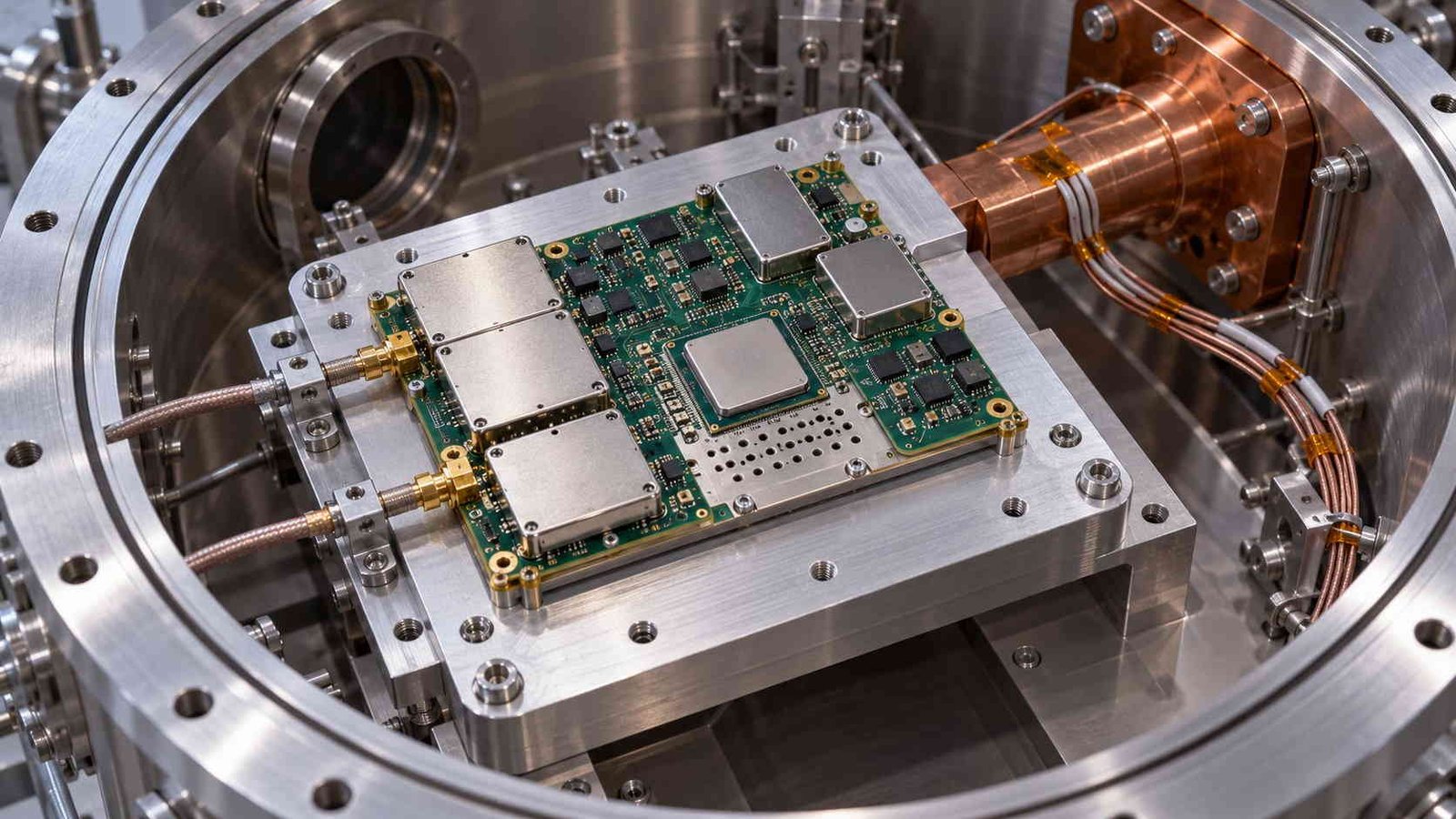
A multi-channel SDR puts two or more receivers and a transmitter in an enclosure the size of a paperback, and then asks for 60 dB of isolation between channels. The board can provide part of that; the enclosure provides the rest. What is almost never checked early enough is that the enclosure is a resonator, and that its first resonance is frequently inside the band.
| Lid or cavity length | First resonance (c/2L) | What sits there |
|---|---|---|
| 30 mm | 5.00 GHz | Top of a 0.5–6 GHz front end |
| 40 mm | 3.75 GHz | Upper C-band |
| 60 mm | 2.50 GHz | S-band, Wi-Fi, telemetry |
| 80 mm | 1.87 GHz | L-band and GNSS |
| 100 mm | 1.50 GHz | Inside the L-band front end |
A shield can is a cavity, and a cavity is a resonator. Computed for an air-filled rectangular lid on its longest dimension; a 100 mm lid puts its first resonance at 1.5 GHz, which is inside the band the board is trying to receive. Shorter lids push the resonance up, and where the geometry cannot change, a lossy absorber on the lid damps the mode instead of moving it.
A 100 mm lid resonates at 1.5 GHz, which is inside an L-band front end; a 60 mm lid resonates at 2.5 GHz, which is inside an S-band one. The fix is not always a smaller box — sometimes the geometry is fixed by the payload — so the practical options are to shorten the cavity with internal walls, to break it into compartments that each resonate above the band, or to damp the mode with a lossy absorber on the lid. What does not work is assuming the lid is a shield and not a cavity.
On the board, the fence is the tool. A via fence at λg/20 holds the boundary of a shielded region: at 6 GHz in a hydrocarbon laminate that is 1.51 mm, at 3 GHz 3.02 mm, at 1.5 GHz 6.04 mm. The number that matters is the highest frequency on the board, not the band of the channel being shielded, because a harmonic or a lane edge will find the gap that the fundamental did not. The fence has to be continuous where the can gasket lands — a fence that exists only at the corners leaves three sides of the cavity open.
Board-level isolation between RF and digital follows three rules that are boring and effective: no parallel runs between domains longer than a twentieth of a wavelength, orthogonal routing where a crossing is unavoidable, and a ground stitch fence along the boundary with vias placed on a pitch that scales with the highest frequency. The mechanism behind the fence — what it does to a radiating edge and where it stops helping — is in our QFN MMIC layout and LNA grounding and shielding guides.
8. Acceptance Data and the Review That Prevents a Re-Spin
A wideband SDR board is expensive to debug because the failures are distributed: 0.3 dB of extra loss at 6 GHz, 10 ps of extra skew on one lane, a cavity mode at 2.5 GHz. None of them shows up in a continuity test, and all of them show up in the chamber three weeks before delivery. The defence is to specify the measurements before the build, on the lot that actually ships, and to make each one traceable to a number in the design budget.
| Data item | Method | Criterion |
|---|---|---|
| Insertion loss per band | VNA, 0.5 / 1.5 / 3 / 6 GHz, per channel | ± 0.1 dB of the model at each point |
| Impedance | TDR coupon, RF and lane coupons | 50 Ω ± 5 %, 100 Ω differential ± 8 % |
| Lane skew | TDR or VNA, intra-pair and lane-to-lane | ≤ 0.2 UI at the specified lane rate |
| Channel isolation | Two-port between adjacent channels, band centre and edges | ≥ 60 dB, or the number the link budget assumes |
| Phase noise / jitter | Signal source analyser at the converter clock input | Integrated jitter inside the allocation |
| Thermal | Thermal vacuum, or a cold-plate equivalent for commercial space | Junction temperatures inside derating at max dissipation |
| Outgassing | ASTM E595, per lot | TML ≤ 1.00 %, CVCM ≤ 0.10 % |
| Via integrity | Microsection plus thermal cycling, −55 to +125 °C | No barrel crack, no measured resistance rise above 5 % |
| Registration | Cross-section, three points per panel | ± 75 µm between the laminate and the FR-4 section |
The first four rows are what an RF fab will normally quote; the rest are what a space program asks for and what a commercial satellite builder should ask for anyway. None of them is expensive to produce on the lot — they are expensive to reconstruct after the fact, which is why they belong in the purchase order rather than in a follow-up email.
The first four rows are the ones to insist on even on a commercial program. Insertion loss per band catches the material substitution that nobody told you about; TDR catches the impedance that drifted when the prepreg batch changed; lane skew catches the routing that was matched on the wrong layer; isolation catches the fence that was drawn but not drilled. Each of them is a coupon measurement, which means it costs a few hundred dollars on a lot and a few weeks on a re-spin.
Three questions belong in every design review before the Gerbers are released. Is every signal layer referenced to a continuous plane, and does any RF or lane cross a split? Is the clock tree's jitter budget written down as four numbers and added in root sum square, or is it a datasheet value? And does the thermal path survive the loss of convection, with a via count that was calculated rather than inherited? A board that answers those three has a chance of passing thermal vacuum on the first attempt.
If the design is earlier than that — still selecting materials or partitioning domains — the parameter comparisons are in the PCB material comparison chart, the impedance and coupon side in controlled impedance RF PCB, the drill and backdrill limits in high frequency PCB drilling capabilities, and the test-data expectations in mmWave PCB VNA testing. Batch consistency for a serial space program is covered in satellite constellation PCB manufacturing, and the inspection regime in RF PCB quality control.
Space-Grade SDR PCB — Frequently Asked Questions
What "space-grade" means, hybrid stackups, jitter at 6 GHz, backdrilling, and the data that should ship with a lot.
What actually makes an SDR board "space-grade" rather than just high reliability?
Four things, and only one of them is about the laminate. The board has to survive thermal cycling with the plated barrels intact, which is a CTE and stackup problem; it has to meet outgassing limits, which is a material and process chemistry problem; it has to get its heat out by conduction because there is no air; and it has to be traceable from laminate lot to shipped serial. A high-reliability industrial board usually satisfies the first and none of the other three. The laminate class is a consequence of those requirements, not the definition.
Can the RF half and the digital half use different laminates on the same board?
Yes — it is the normal arrangement, and a 12-layer SDR board is usually a hybrid of four low-loss layers and eight FR-4 layers. What has to be designed is the seam: registration between the two materials, the z-axis CTE step through any barrel that passes from one to the other, warp over a large panel, and the delay step for any lane that changes medium. The same 100 mm of trace is 552 ps in hydrocarbon and 603 ps in FR-4, so a lane that crosses the boundary without accounting for it loses about 0.5 ps per millimetre of the transit.
How much clock jitter can I afford at 6 GHz?
Work backwards from the bits you actually need. At 6 GHz, 100 fs rms gives 7.8 effective bits, 200 fs gives 6.8, and 500 fs gives 5.4. If you need 10 effective bits at 6 GHz, you need better than 50 fs, and that is an oscillator and clock-tree problem before it is a layout problem. A realistic four-term budget — oscillator 60 fs, buffer 40 fs, supply 50 fs, board 30 fs — adds up in root sum square to about 93 fs, which is 7.9 bits. That number is why 12-bit converters at 6 GHz rarely deliver 12 bits in a system.
Does a 6 GHz SDR board need backdrilling?
Not for the RF section, and that is worth saying plainly because backdrilling is often specified by reflex. On a 1.6 mm board a 1.0 mm stub resonates at 39.5 GHz and represents about 14 degrees at 6 GHz, which is not the limiting discontinuity. What does limit the board at 6 GHz is the connector launch, the reference-plane transition and the filter pad geometry. Backdrilling earns its cost when the same stackup also carries a 15 GHz or higher path, or when the board is thick enough that the stub resonance falls near the operating band.
What test data should ship with each lot?
Insertion loss at the band edges and centre against the model, TDR for impedance and lane skew, adjacent-channel isolation, and a microsection with thermal cycling if the program is space. Add the ASTM E595 outgassing report per laminate lot and the lot-to-lot Dk check on the coupon. The rule we use is simple: if a number appears in the link budget or the thermal budget, there should be a measurement behind it in the lot documentation, not a datasheet value quoted from the material supplier.
Building a wideband SDR or a space-bound RF board?
Send us the band set, the lane rate and the stackup you have in mind. We will confirm the achievable loss and skew spread before the layout is frozen, agree which Dk figure goes into the impedance target, and quote fabrication with coupon TDR, insertion loss and microsection data on the lot we actually build from.
Contact Us → WhatsApp: +86 137 6047 3650Request a PCB Quote
Upload your Gerber ZIP file and project requirements. Our engineering team will review your PCB material, stackup, impedance needs, surface finish, and production quantity before quoting.
Please prepare:
- Gerber files in ZIP format
- PCB material or stackup requirements
- Controlled impedance notes if available
- Prototype or batch production quantity