
RF Power Divider PCB: Wilkinson Networks, Isolation and Balance
RF power divider PCB guide: Wilkinson networks on board, multi-way loss budgets, isolation resistor power, etch tolerance and amplitude/phase balance specs.
Home » Amplitude Phase Balance » RF Power Divider PCB: Wilkinson Networks, Isolation and Balance
Table of Contents
Power dividers rarely headline a system — they sit between the amplifier and the antenna, between the receiver and the channels, between the test port and the DUT. But the discipline they demand is real: a recently reported naval-defense award for divider networks — 2- to 8-way, coherent and non-coherent, spanning DC–40 GHz, with strict amplitude and phase balance and high port-to-port isolation — is the clearest statement of what this passive network has to hold. The same structures, minus the export-controlled wrapper, are the daily bread of commercial radar receivers, switch matrices and RF test systems.
This page computes the board-level conversation: where the multi-way “loss” actually comes from; what a quarter-wave branch looks like at 2, 10, 28 and 40 GHz; how sensitive the 70.7 Ω branch is to etch; what the isolation resistor must survive when a port faults; and why amplitude and phase balance are manufacturing-controlled acceptance lines rather than losses. Every figure is computed on a stated 10-mil, εr 3.48 stackup; the assumptions are stated where they are used.
The antenna-side application of the same quarter-wave mathematics — feeding an array element by element — is treated in our corporate feed network PCB guide, and the array context in the phased array PCB review. This page is about the divider itself: the Wilkinson network, its resistor, and the specs that decide whether it passes.
1. The Divider Family — and Why the Network Lives on the PCB
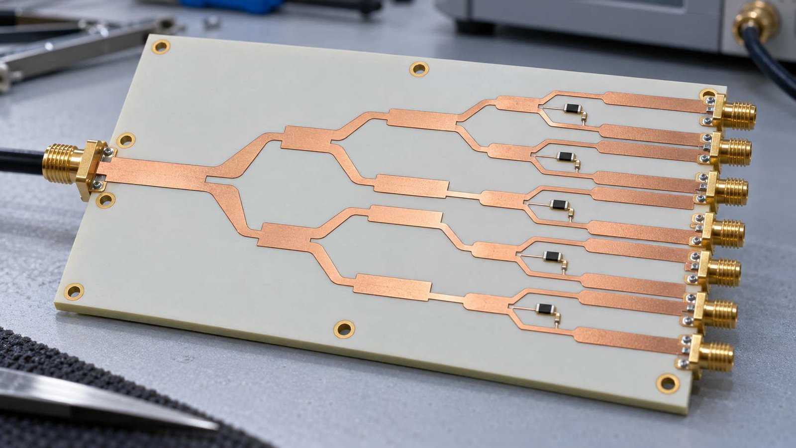
“Power divider” names a family, and the family maps directly onto fabrication decisions. The table sorts it.
| Divider structure on the PCB | How it works | What the fabricator must confirm |
|---|---|---|
| Two-way Wilkinson (single section) | Two λ/4 branches at √2·Z₀ ≈ 70.7 Ω, 100 Ω isolation resistor across the outputs | Branch impedance and λ/4 dimensioned from the agreed stackup, not generic CAD |
| Multi-section Wilkinson | Cascaded λ/4 sections with graded impedances and resistor values for decade-plus bandwidth | Section count vs board area; each section is a controlled-impedance line |
| Multi-way tree (4/8-way) | Cascaded two-way levels; the reported divider class spans 2–8 ways, coherent and non-coherent | Per-level balance stacks — the tree is budgeted level by level, not end-to-end only |
| Resistive divider | Pure resistor network, no λ/4 sections; isolation bought with matched loss | DC-coupled and broadband, but the loss budget is real — instrumentation class |
A recently reported naval-defense award for divider networks — 2- to 8-way, coherent and non-coherent, DC–40 GHz, low insertion loss with strict amplitude and phase balance and high port-to-port isolation, built in an AS9100D-registered plant — describes exactly this family. The defense-program version of it is hard to enter directly; the same structures ship every day in commercial radar receivers, switch matrices and RF test systems, and that is the market this page is written for. The antenna-side relative of this network — the corporate feed that distributes power to array elements — is treated in our corporate feed network PCB guide; this page is about the divider itself as a component.
The row that changes RFQ behaviour is the multi-way tree: cascading two-way levels multiplies not just the loss but the balance budget — each level’s amplitude and phase error stacks through the tree, which is why an 8-way is quoted and verified level by level, not only end to end. The reported 2–8-way, coherent and non-coherent divider class in the naval award covers exactly this span; the commercial versions of the same tree ship in receiver splitters, radar chains and test systems.
2. Multi-Way Arithmetic: Where 9 dB of “Loss” Comes From
The most common procurement misunderstanding starts here.
| Way count | Ideal splitting loss (10·log₁₀N) | What the real spec adds |
|---|---|---|
| 2-way | 3.01 dB | Dissipation of the branches and resistor pads on top — typically a few tenths of a dB |
| 4-way | 6.02 dB | Two stacked levels: branch dissipation adds level by level |
| 8-way | 9.03 dB | Three levels. "Insertion loss" quotes that sit far below 9 dB for an 8-way are quoting relative to ideal, not absolute |
Splitting loss to N matched ports is fixed by physics: 10·log₁₀N. The number that actually compares suppliers is the excess over ideal — branch dissipation, pad parasitics and radiation — and it is measured on a swept band, not read from a single frequency point. When a datasheet in the reported DC–40 GHz class quotes "low insertion loss" for a multi-way divider, the first question is always: relative to what?
Splitting to N matched ports costs 10·log₁₀N — physics, not engineering. So the real comparison between suppliers is the excess over ideal, and it is a swept-band measurement: branch dissipation, pad parasitics and radiation, level by level through the tree. An RFQ that asks for “low insertion loss” without defining the reference gets quotes that are not comparable; an RFQ that asks for excess-over-ideal across the band gets engineering.
3. Quarter-Wave Geometry: the Circuit Is the Drawing
A Wilkinson divider is three dimensions and a resistor: two λ/4 branches at √2·Z₀ ≈ 70.7 Ω and a 100 Ω resistor across the outputs. The table shows what those dimensions become as the band climbs.
| Frequency | λ/4 main line (50 Ω, εeff 2.79) | λ/4 branch (70.7 Ω, εeff 2.62) | Layout consequence |
|---|---|---|---|
| 2 GHz | 22.42 mm | 23.14 mm | Roomy — a single-section Wilkinson fits anywhere |
| 10 GHz | 4.48 mm | 4.63 mm | Standard microwave scale; etch tolerance already a circuit parameter |
| 28 GHz | 1.60 mm | 1.65 mm | Section length is 1.65 mm — layout slack is a phase error |
| 40 GHz | 1.12 mm | 1.16 mm | Broadband at these scales means multi-section, with every section a controlled line |
Quarter-wave lengths computed for a 10-mil, εr 3.48 stackup using the microstrip effective permittivity of each line class (εeff 2.79 for the 50 Ω main line, 2.62 for the 70.7 Ω branch). The table is the whole argument for taking dividers seriously at the fabrication level: at 40 GHz a branch is barely over a millimetre, so the divider lives or dies on line-width control, εr batch stability and launch quality — the same discipline as any mmWave structure in our controlled impedance RF PCB and 50 ohm trace guides.
The 40 GHz row is the argument in one line: a branch barely over a millimetre long. At that scale the divider is not a schematic with a layout attached — it is a set of controlled-impedance lines whose widths, εr batch and launches decide the response, verified on coupons the way any mmWave structure is. The drill-side implication for wideband boards — residual stubs under the branch junctions — follows the same logic as our back drill PCB guide, with depth capability in the drilling capabilities page.
4. Line Width and Etch Sensitivity
The branch is where tolerance concentrates. The table quantifies it.
| Line class (10-mil, εr 3.48) | Synthesized width | ±10 µm etch drift |
|---|---|---|
| 50 Ω main line | 571 µm | ±0.6 Ω (1.2%) |
| 70.7 Ω Wilkinson branch | 316 µm | ±1.1 Ω (1.6%) |
Widths synthesized with the Hammerstad first-order model; the sensitivity is a numerical derivative of that model. Two conclusions follow. First, the thinner 70.7 Ω branch is about twice as sensitive to etch as the 50 Ω main line — etch compensation is set per line class, not per board. Second, at ±10 µm the branch drifts ±1.6%, which is why production verification is a TDR coupon per panel against the agreed stackup, not faith in the nominal width. Etch tolerance and compensation practice are treated in our controlled impedance guide; coupon method in the test fixture guide.
Twice the sensitivity on the branch, twice the reason for per-line-class etch compensation and a TDR coupon per panel. Note what the numbers do not say: ±1.6% impedance drift will not ruin a divider by itself — it eats into a budget that also carries εr batch spread, resistor parasitics and launch quality. That is precisely why the stackup is agreed before layout and verified after etch, in the flow described in our controlled impedance RF PCB guide.
5. The Isolation Resistor: a Power Component Sized for the Fault
In normal operation the 100 Ω resistor across the outputs sees no net power. The fault case is the design case.
| Divider input power | Isolation-resistor dissipation (one port open) | Conventional chip resistor verdict |
|---|---|---|
| 1 W | 0.25 W | 1206 / 2512 chip survives |
| 10 W | 2.5 W | No conventional chip — flanged thin-film termination or metal-carrier resistor |
| 40 W | 10 W | 25× beyond a 1 W 2512 — a thermal design, not a component pick |
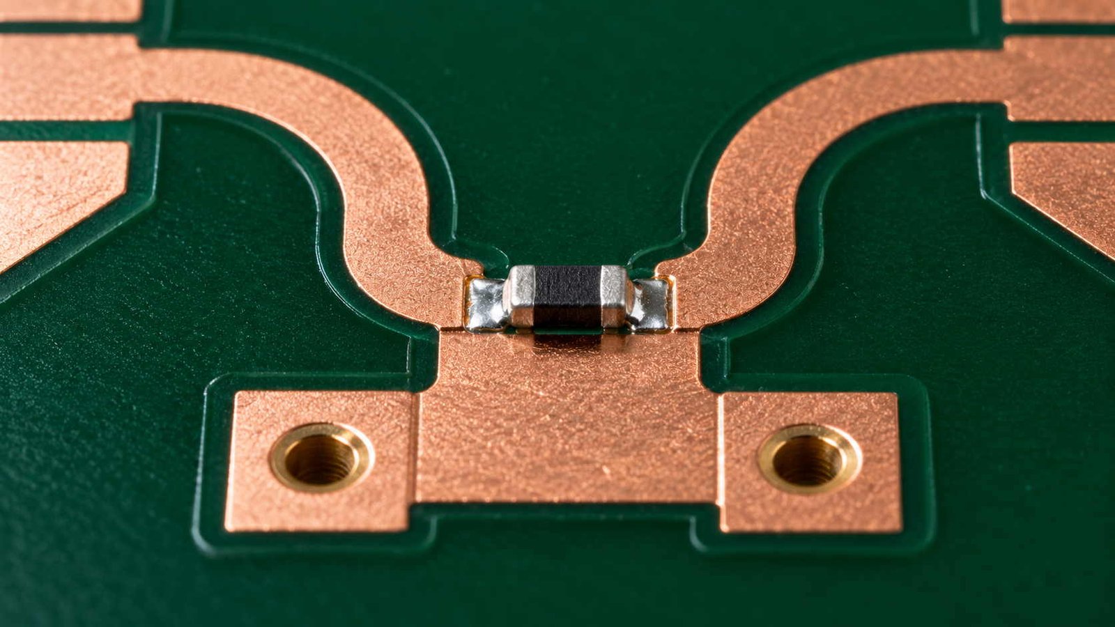
P_iso = P_in/4: with one output open, each branch carries half the input, the reflected wave splits at the isolation node, and one quarter of the input power lands in the 100 Ω resistor. That is the design point — the isolation resistor is sized for the fault case, not the signal case, and its land, heat path and placement belong on the fabrication drawing. On high-power combiner trees the same arithmetic runs in reverse, which is why the combining network and the PA thermal design are one conversation — see our GaN RF power amplifier thermal guide and the RF power amplifier PCB review.
The arithmetic is blunt: one open port sends a quarter of the input power into that resistor. At instrumentation levels a chip resistor is fine; at radar-chain levels the isolation element is a flanged thin-film termination or a metal-carrier resistor with its own thermal path — a decision that belongs on the fabrication drawing, next to the land pattern and the heat-spreading copper underneath. In combiner trees the same network runs in reverse and the power side grows, which is why the combining structure and the PA thermal design are one conversation in our RF power amplifier PCB review.
6. Balance: a Compliance Line, Not a Loss Line
Amplitude and phase balance sound like loss topics. The arithmetic says otherwise.
| Manufacturing variation | Effect on balance | Framing |
|---|---|---|
| Etch ±10 µm on the branch (10 GHz) | ±0.19° phase | Well inside a ±3° spec |
| Etch ±10 µm on the branch (28 GHz) | ±0.54° phase | Still inside spec — but the budget is no longer empty |
| εr batch ±1% | ±0.23° on a 90° section | Why laminate batch control and coupons are part of the balance spec |
| 0.5 dB amplitude imbalance | ≈ 0.003 dB combining loss | Balance is not a loss problem — it is an acceptance-compliance line, typically ±0.3 dB / ±3° with isolation ≥ 20 dB across the band |
Phase effects computed for the 70.7 Ω branch εeff 2.62. The verdict row reframes the whole spec: amplitude and phase balance barely move the loss budget, but they are pass/fail contract lines measured across the band — which makes them manufacturing-controlled parameters: line-class etch compensation, laminate batch data, and swept S-parameter evidence with launch de-embedding rather than spot checks. The measurement method is set out in our mmWave VNA testing guide; ground stitching around the branches in the via fence PCB guide.
The verdict row is the reframe: balance barely moves the loss budget, but it is a pass/fail acceptance line on nearly every divider specification — the reported naval-award family advertises exactly these parameters. Manufacturing answers it with etch compensation per line class, laminate batch data, ground stitching that keeps the branch reference intact, and swept S-parameter evidence with launch de-embedding. The measurement method is set out in our mmWave VNA testing guide; the ground-side stitching pattern in the via fence PCB guide.
7. The DFM Checklist Before the Divider RFQ
Nothing here is exotic; each line traces to a number computed above, and each is cheap on a drawing and expensive to reconstruct after a first article fails acceptance.
| # | Drawing or PO line item | Why it is on the list |
|---|---|---|
| 1 | Branch impedance and λ/4 lengths dimensioned from the agreed stackup (εeff per line class) | The circuit is the drawing (section 3) |
| 2 | Etch compensation per line class; impedance coupon TDR per panel | The 70.7 Ω branch drifts ±1.6% at ±10 µm (section 4) |
| 3 | Isolation resistor: value, power class and heat path sized to the fault case (Pin/4) | A 40 W divider puts 10 W in the resistor on one open port (section 5) |
| 4 | Resistor land pattern and pad parasitics controlled for the band | Pad parasitics are part of the isolation structure |
| 5 | Balance and isolation spec on the drawing: amplitude, phase, port-to-port, all swept | ±0.3 dB / ±3° / ≥20 dB class specs are acceptance lines (section 6) |
| 6 | Multi-way trees budgeted level by level | Per-level imbalance stacks through the tree (section 1) |
| 7 | Ground stitching / via fences along both branches | Reference continuity is half the branch impedance |
| 8 | Swept S-parameters with launch de-embedding on production coupons | Spot-check data proves nothing across DC–40 GHz-class bands |
Eight lines, each tracing to a number computed above. Items 1–4 decide whether the network meets the band; 5–6 decide whether it passes the balance and isolation acceptance; 7–8 decide whether the evidence exists lot by lot. A divider RFQ that carries these eight answers is quotable on engineering.
The pattern across the whole page: a divider is a small network with a large specification surface — way count, band, power, fault case, balance, isolation — and every one of those lines lands on the fabrication drawing. For the adjacent decisions — the array feed that shares the quarter-wave mathematics, the PA chain that sets the power the resistor must survive, or the material families behind the stackup — the corporate feed network PCB guide, the PA design guide, the X/Ku-band AESA radar PCB guide and the PCB material comparison chart are the right starting points, and our RF PCB manufacturer overview covers the fabrication capabilities behind all of them.
RF Power Divider PCB — Frequently Asked Questions
Where the "loss" goes, what the isolation resistor must survive, which structure fits which band, why balance is a manufacturing line, and what the RFQ should contain.
Why does an 8-way divider show 9 dB of loss — is the part bad?
No — splitting power N ways costs 10·log₁₀N by physics: 3.01 dB for 2-way, 6.02 dB for 4-way, 9.03 dB for 8-way, before any dissipation. The comparable number between suppliers is the excess over ideal: branch dissipation, pad parasitics and radiation, typically a few tenths of a dB, measured swept across the band. Any insertion-loss quote for a multi-way divider should state whether it is absolute or relative to ideal.
What does the isolation resistor actually do, and why is it a power component?
The 100 Ω resistor across the two outputs absorbs the difference between them: with identical signals it sees no net power, and the outputs stay isolated. When one port faults — open or mismatched — a quarter of the input power lands in that resistor (P_iso = P_in/4). So a 40 W divider puts 10 W into the resistor under a single-port fault, which no conventional chip resistor survives. The isolation resistor is a power component sized for the fault case, with its heat path on the fabrication drawing.
Wilkinson, multi-section, or resistive — which structure fits my band?
It follows from bandwidth and loss budget, decided at stackup review with the sweep in hand. A single-section Wilkinson is compact and cheap but narrowband; a multi-section Wilkinson trades board area for decade-plus bandwidth with graded impedances and resistor values; a resistive divider is DC-coupled and extremely broadband but pays for isolation in real loss, which suits instrumentation more than transmit paths. The antenna-side corporate feed — same quarter-wave mathematics, different job — is covered separately in our corporate feed network guide.
Why are amplitude and phase balance a PCB manufacturing conversation?
Because the balance numbers are set by geometry and material, not by design intent. A ±10 µm etch drift on the 70.7 Ω branch is ±0.54° of phase at 28 GHz, and a ±1% permittivity batch spread adds about ±0.23° on a 90° section. The raw loss impact is tiny — 0.5 dB of amplitude imbalance costs about 0.003 dB in combining — but balance and isolation are pass/fail acceptance lines, typically ±0.3 dB, ±3° and ≥20 dB across the band. That makes etch compensation, laminate batch control and swept, de-embedded S-parameter evidence part of the deliverable.
What should a power divider PCB RFQ include?
The conditions that change the board: way count and structure (single-section, multi-section, tree), the band and sweep (DC–40 GHz class in the reported divider family), input power and the fault case the isolation resistor must survive, the balance and isolation acceptance limits and their measurement conditions, and the evidence you expect — swept S-parameters with launch de-embedding, impedance coupons per panel, and traceability on laminate batches. Suppliers who ask for these before quoting are pricing engineering, not guessing.
Building a power divider or combiner network on PCB?
Send us the way count and structure, the band and sweep, the input power and fault case, and the balance/isolation acceptance limits. We will review the branch geometry, etch compensation, isolation-resistor heat path and the coupon plan at stackup review, and quote with swept, de-embedded S-parameter evidence to IPC Class 3.
Contact Us → WhatsApp: +86 137 6047 3650Request a PCB Quote
Upload your Gerber ZIP file and project requirements. Our engineering team will review your PCB material, stackup, impedance needs, surface finish, and production quantity before quoting.
Please prepare:
- Gerber files in ZIP format
- PCB material or stackup requirements
- Controlled impedance notes if available
- Prototype or batch production quantity